# Nash Equilibria

A game can be represented by:

* Players $$N = {1, \cdots n }$$
* Actions → players can do something to affect the world
* Outcomes → players’ actions lead to outcomes
* Preferences over outcomes → each player $$p\_i$$ has a preferences / ranking of the outcomes (in terms of utility)

This provides a general, abstract framework for **strategic interaction**.

### Pure Nash Equilibrium

Given everyone else’s actions $$\vec a\_{-i}$$, the **best response** set of player $$i$$ is:

$$
BR\_i(\vec a\_{-i}) = { b \in A\_i | b \in \argmax u\_i(\vec a\_{-i}, b) }
$$

That is, a player $$i$$’s best response can be any of the actions that give him the maximum possible utility, given everyone else’s actions.

An action profile $$\vec a$$ is a (pure) Nash equilibrium if:

$$
\forall i \in N, a\_i \in BR\_i(\vec a\_{-i})
$$

That is, every player has picked their best response given everyone else’s actions. You can also think of it as: each player picks the action as if they were the last one to do so, and they knew everyone else’s actions.

> *Every player thinks “I’m doing the best I can, given everyone else’s actions.”*

### Mixed Nash Equilibrium

Instead of choosing a single action, one can play a random mix of them (to be unpredictable, otherwise if someone knows you well): $$\vec p\_i \in \Delta(A\_i)$$ is a probability distribution (from the set of all possible probability distributions) over player $$i$$’s actions.

(Note: In general, we use $$\Delta(X)$$ to represent the set of all possible distributions over X)

A (not necessarily pure) strategy profile can be represented as:

$$
\vec p = (\vec p\_1, \cdots, \vec p\_n) \in \Delta(A\_1) \times \cdots \times \Delta(A\_n)
$$

Then, a player’s utility (for a given mixed strategy) is given by:

$$
u\_i(\vec p) = \sum\_{\vec a \in A} u\_i(\vec a)\Pr\[\vec a] = E\_{\vec a \sim \vec p}\[u\_i(\vec a)]
$$

In particular, note that the player’s ONLY care about the **expected value** of their strategy, NOT the variance / risk that their strategy runs. e.g. they would be indifferent to a strategy that guarantees them $50 vs. flipping a coin for $100  — both have the same expected value, and being “risk-neutral”, they wouldn’t care which one they did. That is, they are neutral / indifferent to risk → they don’t care if they take risk or don’t (they don’t avoid it - by taking the gauranteed money - nor do they seek it - by taking the coin flip; they’re just indifferent).

Then, $$\vec p$$ is a (not necessarily pure) nash equilibrium is when: for all players $$i \in N$$, and all possible strategy (possibly containing mixed actions) of each player $$q\_i \in \Delta(A\_i)$$, $$u\_i(\vec p) \geq u\_i(\vec p\_{-i}, \vec q\_i)$$ → their current strategy is at least as good as any other.

In these notes, we use “action” to refer to a pure strategy (only one possible action, played with probability = 1), and the general term “strategy” to refer to possibly mixed actions (i.e., playing multiple actions, each with some probability)

{% hint style="warning" %}
**Nash’s Theorem**: Unlike a *pure* Nash Equilibrium, a (not necessarily pure) Nash Equilibrium ALWAYS EXISTS.
{% endhint %}

The way to compute nash equilibria in a 2x2 games (2 players, each have 2 actions) is by considering 2 possible cases:

1. Case 1 → Compute all NE (if any) in which at least one player plays a pure strategy (do this exhaustively, e.g. “row player plays action X while col player mixes between A and B with probability q and (1-q), then find the value(s) of q for which the best response is X — then you’ve found a NE)
2. Case 2 → Compute all NE (if any) in which both players mix between both strategies

Nash’s theorem says that the union of the set of NE’s found in case 1 and case 2 is non-empty → it doesn’t say whether the NE is pure / not.

The key idea behind case 2 is that the only time that a player would mix between 2 strategies is when (given the opponent’s strategy), he is indifferent to his 2 actions. That is, no matter what action he picks, his utility is the same *given the opponent’s strategy*. This allows us to equate the expected utilities of the two actions for player 1, to find the “mixing probabilities” for player 2 😲 (and vice versa).

### Dominant Strategies

We say that a strategy $$\vec p \in \Delta(A\_i)$$ (weakly) dominates $$\vec q \in \Delta(A\_i)$$ if:

$$
\forall \vec p\_{-i} \in \Delta(A\_{-i}) : u\_i(\vec p\_{-i}, \vec p) \geq u\_i(\vec p\_{-i}, \vec q)
$$

In words: no matter what everyone else does, picking $$\vec p$$ is at least as good as picking $$\vec q$$.

**Strict** domination is when $$u\_i(\vec p\_{-i}, \vec p) > u\_i(\vec p\_{-i}, \vec q)$$ for every $$\vec p\_{-i}$$ → no matter what everyone else does, strategy $$\vec p$$ is STRICTLY better than $$\vec q$$ (and so, you should never even consider picking $$\vec q$$ !!).

{% hint style="warning" %}
**Theorem**: If an action $$a \in A\_i$$ is STRICTLY dominated by some strategy $$\vec p \in \Delta(A\_i)$$, then action $$a$$ is NEVER PLAYED with any positive probability in ANY Nash equilibrium.
{% endhint %}

Intuitively, if you would move all the probability out of the lamer / weaker actions into the ones that dominate it, and you strictly increase your utility. Hence, picking $$a$$ (with any non-zero probability) can never be a “best” response 🤯

**Iterated Removal of Strictly Dominated Strategies**

If you’re trying to find Nash Equilibria, then you can remove action profiles that contain a strictly dominated strategy (from either player’s side).

Note:

* This ONLY works if the action is *strictly* dominated by another strategy (can be a strategy involving multiple actions — using mixed probabilities too)
* If you’re left with a single action / strategy profile at the end, then by Nash Theorem, it must be a NE.
* The reason this works is simply because those cells which contain a strictly dominated strategy (from either player’s side) are never going to happen, i.e., they can never be an equilibrium (because at least one player would change their strategy to the one which strictly dominates it)
* When considrering whether a strategy $$S$$ (may be mixed) strictly dominates an action $$P$$ for the row player, we don’t have to consider all possible strategies of the col player — we can just look at the individual actions and ensure that $$S$$ strictly dominates $$P$$ for every action. Then, since any strategy is a linear combination of actions, if $$S$$ strictly beats $$P$$ for every action of the col player, then $$S$$ strictly beats $$P$$ for every strategy involving those actions too. (Moreover, we only have to lok at the actions of the col players that are not already strictly dominated by other strategies — since col player would not play the weaker actions otherwise).


# Auctions and Routing Games

## Auctions

There are many kinds of auctions all around us:

* Single Item Auction → seller has 1 object, which bidders compete to purchase
* Multi-unit Auction → seller has several identical items for sale, and each bidder wants to get one or more units
* Combinatorial Auction → seller has several distinct items for sale, and each bidder is interested in some combination of items (and the values need not be additive)

The important framework here is:

* Each player / bidder has some internal (”true”) valuation for the item(s).
* Seller decides on the price to sell the item(s).

💡 For every auction, when you design an algorithm / mechanism, you need to answer 2 questions:

1. What is the outcome? i.e., who gets what?
2. What is the payment? i.e.,, who pays what?

### Vickery (Second-Price) Auction

Each bidder $$i \in N$$ values the item at $$v\_i$$.

There are many different formats for the auctions, but we’ll focus on the sealed-bid auction — where all bidders simultaneously submit their bid, and in particular, the vickery-style auction where the highest bidder wins (outcome) and pays the second highest bid (payment).

Then, this can be viewed as a strategic game with:

* $$n$$ players
* players can place bids (these are the actions) — continuous action space
* payoff: if a player values the object at $$v$$ and the 2nd highest bid is $$p$$, then her payoff is:
  * $$v-p$$ if she gets the object
  * $$0$$ if she does not get the object

One might ask: why does the winner pay the second highest bid (and not his / her own bid)? It tunrs out that:

{% hint style="warning" %}
**In a Vickery Auction, truthful bidding is a (weakly) dominant strategy.**
{% endhint %}

That is, a player will not regret telling the truth (reporting her true value as the bid)

So, players have no incentive to lie (i.e., this kind of an auction incentivizes bidders to reveal their true valuations — makes it easy for players to bid since they don’t have to think too much, just be honest) — how amazing would it be if we could make honesty a dominant strategy IN LIFE??

Note: this only applies when players cannot collude with each other.

Also remember that the algorithm / framework never knows what the true valuations of the bidders are — it only sees the bids. But since truthfulness is weakly dominant, it can reasonably *assume* that the bids it sees are the players’ true valuations (since players are assumed to be selfish and greedy).

The proof of this is quite simple (read slides).

All in all, telling the truth is at least as good as any other action.

However, note that there are many nash equilibria in a vickery auction, not just the one where everyone players the dominant strategy of being honest. e.g. $$v\_1 = 50, v\_2 = 70$$. Then, we have the following NEs:

* $$b\_1 = 50, b\_2 = 70$$
* $$b\_1 = 0, b\_2 = 70$$
* $$b\_1 = 70, b\_2 = 0$$

Observe that in the second and third NEs, the auctioneer makes no profit.

The reason we need to cleverly engineer such an auction format — second-price auction — is because in the usual “first price auction” (highest bidder wins, and pays his bid), truthfulness is not dominant, and so, players have incentive to lie (and hence, the mechanism / algorithm cannot actually ensure that the outcome maximizes total value of all players). e.g. if you value the item for $$100$$ and you bid 100, even if you win, your utility would be (value - payment) = 100 - 100 = 0. In fact, *truthfulness is weakly dominated* by a strategy that bids strictly less than your valuation. e.g. bid $$90$$ and pray that others’ bids will be lower, so you make 10 with some probability $$p$$ and $$0$$ with probability $$1-p$$. Also, precisely because of this problem of trying to maximize expected value, you don’t know how much to bid — causes a lot of stress to players trying to optimize their bids (by analyzing other people and their potential valuations). Moreover, it’s possible for the item to be given to someone who (truly) values it less than another person, as a result — so the “total value” in society is not maximized. It’s not “pareto efficient”, since the other person can actually pay more to the guy who got the item and everyone is better off.

This shows the importance of cleverly designing a payment mechanism.

### Multi-Unit Auction

Now, suppose we have $$k \leq n$$ identical items for sale. Each bidder $$i \in N$$ wants one item, and values the item at $$v\_i$$.

What is the analog of Vickrey auction that ensures bidders submit truthful valuations (and so, the mechanism can maximize social welfare by allocating the items to people who value it the most)?

It turns out that we can use a similar reasoning to design the payment structure as follows: each of the top $$k$$ bidders gets the item, and pay the $$(k+1)$$th highest bid.

(Once we discuss VCG, we can show that this payment structure is a specific example of VCG for multi-unit auction — each player pays the “externality” he imposes on others).

Intuitively: everyone who gets the item should be paying the same amount, since they received the same identical item — otherwise, it’s not “fair” (and it wouldn’t be a Nash Equilibria either, since people would try to lower their bids to pay less). e.g. if you asked the top bidder to pay the second highest bid, the second highest bidder to pay the third highest bid, and so on, that wouldn’t incentive honesty. Because I would try to be the kth highest bidder, and once I’ve seen everyone else’s bids, if I am the highest bid, I would want to lower my bid such that im the kth highest bidder, to pay the least and maximize my utility. So, being honest would not be in my interest in this case.

The two main desirable properties of any auction mechanism is that:

* Truthful bidding is a dominant strategy → so that the mechanism can assume the bids are the true valuations and then maximize total utility.
* Items are allocated to the $$k$$ highest bidders → so that the mechanism “tries” (based on the bids at sees) to maximize total social utility.

If we can get both properties, then the mechanism can *assume* that everyone is reporting their true values, and it can maximize the total value to everyone (called “social welfare”), *including the auctioneer*.

### Vickrey Clarke Groves (VCG) Mechanism

In general, mechanism design consists of:

* $$N$$ players from $${1, \cdots, n }$$
* Outcomes $$O = o\_1, \cdots, o\_m$$
* Each player has a valuation function $$v\_i : O \to \mathbb{R}$$
* The algorithm can sometimes assign payments $$\pi\_1, \cdots \pi\_n$$ to each player. Then, a player’s utility for an outcome $$o$$ is given by $$u\_i(o) = v\_i(o) - \pi\_i(o)$$
* The mechanism chooses some outcome $$o^*$$ to maximize some function (called “social choice” function). e.g. utilitarian → $$\sum\_i v\_i(o^*)$$, try to maximize total “social welfare”

Some desirable properties of a mechanism:

* Incentive Compatibility → reporting your true valuations is a NE. That is, If everyone is being honest, your best choice is to be honest too. Hence, everyone is aligned on the incentive to say the truth.
* Dominant Strategy Incentive Compatibility → reporting your true valuations is a (weakly) dominant strategy. That is, *no matter what other people do*, you could always guarantee that being honest is a best response and you won’t regret it.
* **Reason why we use “value” in social welfare, and not utility** The reason “social welfare” in an outcome $$o$$ is defined as the total value of all players under that outcome $$o$$ and NOT total *utility* is quite subtle (yet gives a deeper understanding once you understand it). We also want to consider the auctioneer’s utility. And so, the payment from the bidders goes to the auctioneer, and we can treat the auctioneer’s utility as the sum of all the payment he receives (minus some constant amount that he thinks the items are worth, but that doesn’t matter much). And since the total MONEY in circulation remains the same (just gets transferred from one player to another, in this case the auctioneer), we can actually ignore all payments (and forget above the auctioneer), and focus on maximizing the total value of all the bidders. More formally, let there be $$n$$ players (labelled $$1 \cdots n$$), and 1 auctioneer (labelled 0). Then, if we define social welfare as the total utility of everyone, including the auctioneer, we have:

  $$
  (p\_0 - v\_0) + \sum\_{i=1}^n (v\_i - p\_i)
  $$

  where $$v\_i$$ is the value of the object to person $$i$$, and $$p\_i$$ is the amount paid by player $$i$$ under the mechanism (and the auctioneer RECEIVES the payment and GIVES the item, so we need to flip the utility function) This also shows us that if the auctioneer values the item at $$v\_0 > \max\_{i \in {1, \cdots, n}} p\_i$$, he should not give it away — he derives more value keeping it than receiving the payment. But okay, suppose that this is not the case, and that the auctioneer gives away all the objects. Observe, that the amount the auctioneer receives is exactly how much the bidders pay (duh). So, $$p\_0 = \sum\_{i=1}^n p\_i$$. And then, we can simplify social welfare to:

  $$
  (\sum\_{i =1}^n v\_i)- v\_0
  $$

  where player $$i$$ receives “value” $$v\_i$$ from the object, and 0 if they don’t get the object. And since $$v\_0$$ is a constant that does not depend on the allocation of the items among the $$n$$ bidders, we can ignore it when trying to maximize social welfare. HENCE, we can focus on maximizing the total value gained by the bidders alone. (Of course, if we’re considering utility we need to include the auctioneer because if not, he will end up with nothing LOL i.e., if we only consider maximizing bidders’ utility then optimally, the top k bidders get the items and pay nothing for it — and since they pay nothing, it doesn’t even incentivize truthfulness, and so, we aren’t really maximizing bidder’s “true” utility since we can’t reasonably assume that their bids = valuations. Understand the line of reasoning. This is why it’s important to be very careful while designing mechanisms to ensure incentives align with what you want to achieve).

The VCG mechanism is a general framework of truthful mechanisms. It selects socially optimal outcome, and ensures truthful reporting by careful payment design.

In fact, it can only maximize (real) social welfare under the assumption that it receives honest valuations from players, and this assumption is reasonable *because* the payment designs makes truthfulness a dominant strategy → the logic of WHY VCG works is important! So, the only assumption we’re really making is that players are selfish and greedy, i.e., they care about maximizing their OWN utility, not the joint utility of all players. This is the genius of VCG.

VCG Procedure:

* Outcome: Choose some outcome $$o^*$$ that maximizes $$\sum\_i v\_i(o^*)$$ → hence, $$o^\*$$ is socially optimal.
  * Payment: Each agent pays the **externality** that she imposes on the other agents. That is, how much value is she “taking” away from the other players by being present. Let $$o\_{-j}^\*$$ be the outcome that maximizes $$\sum\_{i \neq j} v\_i$$ → i.e., the social welfare of others in the absence of player $$j$$. Then, player $$j$$ pays: (max welfare of others if j were obsent) $$-$$ (max welfare of others when j is present) which is:

    $$
    \sum\_{i \neq j}\[v\_i(o\_{-j}^*) - v\_i(o^*)]
    $$

Using this, we can show that Vickery auction is a special case of VCG (as is the multi-unit auction format where each of the top $$k$$ bidders pays the $$(k+1)$$th highest bid, because that’s the externality they impose — in their absence, the $$(k+1)$$th bidder would’ve gotten the item but you “took” it from them so you must pay that much).

{% hint style="warning" %}
**In VCG mechanisms, truthful reporting is a dominant strategy.**
{% endhint %}

This is the whole point of VCG! And it’s not obvious at first glance.

Remember:

* The mechanism only sees the bids — it maximizes social welfare *assuming the bids represent honest valuations*. But the assumption is just necessary to intrepret what the algorithm is doing — the algorithm just treats the bids as numbers and maximizes a function. In particular, if $$w\_{ik}$$ is player $$i$$’s bid for item $$k$$ (assuming we have many items), then the mechanism maximizes $$\sum\_k \sum\_i w\_{ik} \cdot I(i, k)$$ where $$I(i, k)$$ is the indicator variable that represents whether player $$i$$ received item $$k$$ or not.
* In theory, the mechanism never knows whether the bids were honest or not. So, the mechanism cannot calculate any individual’s “utility”. That is, each person’s utility function is private to them since only they know their true valuations. BUT while analyzing the mechanism, we can assume we know everyone’s utility functions by looking into the minds of each bidder, since each individual knows her utility function. And by misreporting, she doesn’t change her true valuation — yes, the mechanism gets a different input and might pick a different outcome, but the individual knows her utility function hasn’t changed. e.g. if $$v\_i = 10$$ but you bid $$w\_i = 100$$ and have to pay $$50$$ to get the item, your utility is $$-40$$, not $$50$$.
* If there are multiple possible outcomes that have the same social welfare, then it can be shown that no matter which one is picked, the utility of each player doesn’t change.

Okay, let’s prove that honesty is the best policy here.

Let $$w\_i$$ be the bid of player $$i$$. Then, the utility of player $$j$$ when she reports truthfully is given by:

$$
v\_j(o^*) - \left(\sum\_{i \neq j} w\_i(o\_{-j}^*) - \sum\_{i \neq j} w\_i(o^\*) \right )
$$

Note that player $$j$$ cannot affect the other players’ bids. That is, we actually only ask the players for bids ONE time — we don’t actually remove each player, and ask the other players to report bids. So, the bids of other players don’t depend on player $$j$$’s reported bids (since they don’t even see each other’s bids).

Note that $$v\_j$$ is a constant. And by definition, $$o\_{-j}^\*$$ does not depend on $$j$$’s report.

So, we have:

$$
\sum\_{i \neq j} w\_i(o\_{-j}^*) + \sum\_{i \neq j} w\_i(o^*) + v\_j(o^\*)
$$

Now, the mechanism is defined in a way to find a $$o^*$$ that maximizes $$\sum\_i w\_i(o^*)$$.

And so, for player $$j$$’s incentive to align with what the mechanism is doing, he should report his true value.

> I think it takes a while to really get this — write it down on a piece of paper. See that it doesn’t matter what the other players do i.e., we don’t have to assume other players are being honest, in fact no one will ever know if the players were honest or not (since no one can know the true valuations of anyone else) - the mechanism is just a maximizing function.

### Combinatorial Auctions

We have $$m$$ possible distinct items for sale, and $$n$$ bidders.

So, we have $$(n + 1)^m$$ possible outcomes → for each item, we can either give it to one of the bidders or not give it to anyone (i.e., keep it with the auctioneer).

Bidders can have different valuations for different subsets of items — importantly, the valuations don’t have to be additive. I can value a notebook for $$10, and a pen for$$2, but the combination for $$15 - since they both become more useful to me when I have both.

VCG still works, and ensures truthfulness but we have some challenges:

* Preference elicitation: Each bidder has $$2^m$$ private parameters.
* Computational issues: Finding the optimal outcome $$o^\*$$ may be NP-hard (it’s basically like knapsack)
* Revenue non-monotonicity. That is, adding more bidders can cause the payment (to the VCG mechanism / auctioneer) to decreases, which is very counter-intuitive but true (since it’s possible for a group of bidders to be imposing an externality but none of them individually are). e.g. 2 items (A, B). 2 players (X, Y). X values {A,B} at 10, but values {A} = {B}= 0 (he only wants them together, or not at all). Player Y only values {A} = 11. So, VCG assigns {A} to Y, and Y pays 10. Now, if a player Z enters and values {B} = 11, then player Y still gets {A} and Z gets {B} but both of them pay nothing (because even if Y / Z were absent, the other player would “block” X from getting the “combo set” — so each person’s individual externality is zero).

### Routing

#### Non-Atomic

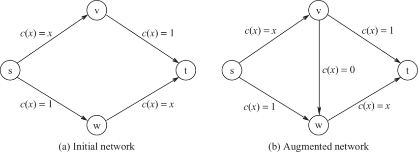
Braess’s Paradox: Adding an edge (even a magical edge with no cost) can lead to a worse equilibirum since everyone rushes to use that edge. Not just worse off overall, but worse for every individual.

(Adding an edge can NEVER increase the optimal cost.)

<figure><img src="https://2994438412-files.gitbook.io/~/files/v0/b/gitbook-x-prod.appspot.com/o/spaces%2FixDr0QrEmvZAtfJXNbfW%2Fuploads%2Fwz0M77HQLk4kzsgSWQ8B%2Fimage.png?alt=media" alt=""><figcaption></figcaption></figure>

In (a) due to obvious symmetry, half the people take the top route and half take the bottom route. Then, the total time for everyone is 1.5 hours (assuming we have one unit of traffic to route, and it is non-atomic).

In (b), everyone would like to go through s → v → w → t, since time x < 1 for any x (until everyone goes through this path). And then, we end up in a situation where everyone takes 2 hours.

The optimal solution here would be to allocate half of them to go via the first route and the other half via the second half.

This is kind of like the prisoner’s dilemna. People try to be selfish and only think of their own utility, leading to a worse situation for everyone (not just *everyone else*, but everyone!). Of course, the reason this is an equilibrium is that everyone is thinking of themselves, and given that everyone is selfish, your best response is also to be selfish.

The key insight here is that selfish behaviour hurts social welfare. We can measure “how much” it hurts social welfare by finding the “Price of Anarchy”.

**Price of Anarchy** is defined to be the ratio of the social cost under the worst Nash Equilibrium and the socially optimal solution.

$$
PoA = \frac{WorstNash(G)}{OPT(G)}
$$

It’s called price of anarchy because the worst Nash equilibrium is the worst-case “stable” state that the people can arrive at with no central authority to force them to do anything. But oftentimes, if we have a central authority that can decide who does what, we can get a better overall outcome (for society) — though not necessarily for every person (some people may have to sacrifice for the overall good). So, the freedom (aka anarchy) comes at a cost (aka price) to everyone.

**In non-atomic (you can split as finely as you want) routing games, all equilibrium flows have the same cost, so we we can take any equilibrium in the numerator above.**

### Atomic Version

Suppose we have $$k$$ units of traffic, where $$k$$ is a positive integer. Each unit must be routed as a whole (think of each unit as a car).

Each edge $$e \in E$$ has a cost function, $$c\_e : \mathbb{N} \to \mathbb{R}\_{\geq 0}$$.

**In an atomic routing game, a PURE Nash equilibrium flow always exists.**

That is, no player needs to pick routes randomly (in a “mixed actions” way) — he/she can pick a single route, given other people’s choices.

Note that this does NOT follow directly from Nash’s theorem — Nash only says that there exists AN equilibrium, it doesn’t have to be pure. So, this is a stricter condition, and one that is not implied by Nash.

Proof: We can show that every atomic routing game is a **potential game**. And all players are inadvertently (unknowingly / unintentionally) and collectively striving to optimise a **potential function** $$\Phi$$**.**

The cleverness of this proof lies in this choice of potential function(!!), just like the cleverness of VCG lies in their payment design.

$$
\Phi(f) = \sum\_{e \in E} \sum\_{i = 1}^{f\_e} c\_e(i)
$$

where $$f\_e$$ is the number of players that chose a path that includes the edge $$e$$.

This choice of potential function is not obvious. In particular, note that this doesn’t capture the total cost of everyone — that would be given by: $$\sum\_{e \in E} f\_e \cdot c\_e(f\_e)$$ since each of the $$f\_e$$ players using that edge would incur a cost of $$c\_e(f\_e)$$.

But the crucial property is that: If a player deviates from path P to $$\hat P$$, the change in the potential function is:

$$
\Phi(\hat f) - \Phi(f) = \sum\_{e \in \hat P} c\_e(\hat f\_e) - \sum\_{e \in P} c\_e (f\_e)
$$

That is, remove the contribution of this player to the potential when they were using path $$P$$, and then, add the contribution back based on the path $$\hat P$$.

BUT, this is exactly the change in the deviator’s individual cost! In other words, when a player deviates, the change in the potential function is the same as the change in the deviator’s individual cost!

So, a flow that minimizes the potential function is an equilibrium. Hence, we’re done.

Umm.. why are we done? Because out of all the flows, just pick a (not necessarily unique) one with the minimum potential. And that is going to be an equilibrium because no player has any incentive to deviate (if they did, they would do so, and decreasing their cost would also lower the potential function, but by definition, this is the minimum potential value, so its not possible).

A similar proof works for non-atomic routing games - by using integral instead of sum over the cost function.

So, we’ve proven (using the potential function argument) that a *pure* nash equilibrium flow always exists.


# Cooperative Games

## Cooperative Games

Players divide into coalitions to perform tasks. Within a coalition, members can freely divide profits. The question is how should the profits be divided?

### Induced Subgraph Games

<figure><img src="https://2994438412-files.gitbook.io/~/files/v0/b/gitbook-x-prod.appspot.com/o/spaces%2FixDr0QrEmvZAtfJXNbfW%2Fuploads%2FJH2CRlncFLQgc1rxQO26%2FScreenshot_2024%2009%2012_at_5.42.43_PM.png?alt=media" alt=""><figcaption></figcaption></figure>

We are given a weighted graph where the players are nodes; and the value of a coalition is the value of the total edge weights in the subgraph.

So, an edge $$(u,v)$$ tells you how much value $$(u,v)$$ would generate if they work together. e.g. researchers collaborate to each other (and the total value is determined by the sum of their pairwise values).

(And it seems natural / intuitive to assume that if $$(u,v) = k$$ then each of $$u$$ and $$v$$ contribute $$k/2$$ to this synergistic “relationship”).

### Network Flow Games

<figure><img src="https://2994438412-files.gitbook.io/~/files/v0/b/gitbook-x-prod.appspot.com/o/spaces%2FixDr0QrEmvZAtfJXNbfW%2Fuploads%2F9f8PGpNbjz2Lc0rxtda2%2FScreenshot_2024%2009%2012_at_5.42.56_PM.png?alt=media" alt=""><figcaption></figcaption></figure>

We are given a weighted directed graph. Players are edges. And the value of a coalition is the value of the maximum flow it can pass from $$s$$ to $$t$$. This has applications in computer network, traffic flow, transport networks. (that is, the minimum bottleneck value on the path).

### Weighted Voting Games

We are given a list of weights and a threshold, i.e., $$(w\_1, \cdots, w\_n; q)$$, all of which are positive integers. Each player $$i$$ has a weight $$i$$.

The value of a coalition is 1 (winning) if its total weight is at least $$q$$ (winning), and 0 (losing) otherwise.

Applications: parliaments, UN security council, EU council of members.

{% hint style="info" %}
Cost sharing is just the inverse of profit sharing. So it’s actually the “same” problem underneath the hood — if you have an algorithm that can fairly divide profits, you can negate the values to convert them to costs (i.e., change maximization to minimization).
{% endhint %}

### General Framework

* A set of players - $$N = {1, \cdots, n }$$
* A valuation function - $$v : 2^N \to \mathbb{R}\_{\geq 0}$$
  * That is, each subset of players have some value associated with it (and that’s the value of the group). Here, $$2^N$$ just denotes the power set of $${1, \cdots, n}$$
  * $$v(S)$$ is just the value of a coalition $$S$$, and by default, $$v(\phi) = 0$$
* Coalition structure (CS) → a partition of $$N$$ (into groups) — each person is in exactly one coalition.
* We aim to find the optimal coalition structure — the structure that maximizes total generated value from the $$n$$ players. That is, $$OPT(G) = \max\_{CS} \sum\_{S \in CS} v(S)$$
* But we also need to satisfy some (reasonable if you think about it) constraints:
  * **Efficiency**: a vector $$\vec x \in \mathbb{R}^n\_{\geq 0}$$ satisfying $$\sum\_i x\_i = v(N)$$
    * Basically this says that each person gets 1 number, which is their payoff, and the total value that the group generates must be completely distributed among the $$n$$ people.
    * It’s called efficiency because there’s no loss in value. Whatever value is generated is distribued without any loss. Nothing is kept for the mechanism or wasted. It’s a matter of economic efficiency — no one can improve without anyone else being hurt — and has nothing to do with computational efficiency.
  * **Individual Rationality**: $$x\_i \geq v\_i$$ for all $$i \in N$$
    * You need to give each person at least how much value they would generate by being alone — if not, they will leave your group (”deviate”), and do their own thing.
* An **imputation** is just a vector that satisfies efficiency and individual rationality.

### Cooperative Game Properties

A game $$G = \<N, v>$$ is called:

* **Monotone**: for any $$S \subseteq T \subseteq N$$, $$v(S) \leq v(T)$$
  * Adding anyone cannot decrease the value of the coalition.
* **Simple**: if $$G$$ is monotone AND $$v(S) \in {0, 1}$$
  * i.e., the value of any coalition is binary, winning or losing, and adding anyone to a winning coalition cannot make the coalition lose (there’s no snitch :O)
* **Superadditive**: for disjoint $$S, T \subseteq N$$, $$v(S) + v(T) \leq v(S \cup T)$$
  * collaboration is always beneficial to the overall value generated
* **Convex**: for $$S \subseteq T \subseteq N$$ AND $$i \in N \setminus T$$, we have $$v(S \cup {i}) - v(S) \leq v(T \cup {i}) - V(T)$$
  * the marginal gain of player $$i$$ by adding to $$S$$ cannot be more than the marginal gain if player $$i$$ joins $$T$$, and $$T$$ contains at least everyone in $$S$$ (and possibly more) — because the opportunities to collaborate is more. (joining a bigger group is always better, given that one is a subset of the other)

Monotone $$\land$$ Convex $$\implies$$Superadditive.

## Dividing Payoffs in Cooperative Games

### The Core

An imputation $$\vec x$$ is in the core if:

$$
\sum\_{i \in S} x\_i = x(S) \leq v(S), \forall S \subseteq N
$$

That is, each susbet of players is getting at least what it can make on its own.

It’s easier to think about what would happen if we did not satisfy the above criteria. Then, a subset of players are together being paid less than the value they bring to the table. So, they would deviate from the group (making it unstable) and divide the profits among themselves in a way that they at least get as much as they were getting before, with some people getting more now.

So, being in the core is a notion of stability: no subset of players have any incentive to deviate.

So, the core is a set of vectors that satisfies the linear constraints:

* $$\sum\_{i \in N} x\_i = v(N)$$ — the total payoff given to everyone is equal to the total value they generate.
* $$\sum\_{i \in S} x\_i \geq v(S), \forall S \subseteq N$$ (by definition of being in the core)

Also, remember:

* **x**$$(S)$$ is additive in the sense that the total payoff of a group is the sum of the individual payoffs given to each person (think of it as cash).
* BUT $$v(S)$$ is not additive — otherwise there would be no point in collaborating and this would be a boring problem. They can generate more / less value as a group than individually (think of synergy, 1 + 1 > 2)

<figure><img src="https://2994438412-files.gitbook.io/~/files/v0/b/gitbook-x-prod.appspot.com/o/spaces%2FixDr0QrEmvZAtfJXNbfW%2Fuploads%2FRi1JaFzYDKptATI67MXc%2FScreenshot_2024%2009%2012_at_6.09.42_PM.png?alt=media" alt=""><figcaption></figcaption></figure>

For a 3-player game, we can find the core by drawing a triangle, and then each point on the triangle maps to a payoff vector. e.g. the top vertex means that all the payoff goes to the first player. The midpoint of the bottom edge means that the payoff vector is $$\vec x = (0, \frac{v(N)}{2}, \frac{v(N)}{2})$$. In general, each person gets paid in the inverse of the ratio of the distance from the point to the edge opposite that player’s vertex.

### Is the Core Empty?

A natural question to ask then is: is the core empty?? That is, is there ANY possible payoff vector that ensures that no subset of players deviate?

**Simple Game**: A game is called simple if $$v(S) \in {0, 1}$$ for all $$S \subseteq N$$ and it is monotone (adding players to a coalition does not decrease the value).

Coalitions with value 1 are winning. Coalitions with value 0 are losing.

A player is called a a veto player if she is a member of every winning coalition (can’t win without her).

💡 **Theorem: Let** $$G$$ **be a simple game then** $$Core(G) \neq \phi \iff G$$ **has veto players. In fact, the core has precisely the vectors that distribute the payoff ONLY among the veto players.**

The proof is relatively simple: if we give any positive payoff to a non-veto player, then the remaining players can deviate together (and they can divide this positive payoff among themselves).

If we give positive payoff ONLY to veto players, then since any winning coaliion must contain ALL veto players, there is no benefiical deviation. BUT notice that this doesn’t mean that we have to give every veto player the same payoff, or even that we have to give every veto player a positive payoff(!!). So, ANY distribution of the payoff among only the veto players is in the core (no subset of players can deviate).

💡 **Theorem: For an induced subgraph game, the core is not empty** $$\iff$$ **the graph has no negative cut.**

In particular, if the core is not empty, a possible payoff strategy is the *shapley value* which assigns each node half the value of the edges connected to it.

Let’s prove the theorem.

* ($$\impliedby$$) If there is no negative cut, then the core is not empty.
  * It suffices to find 1 payoff vector in the core.
  * Let $$\phi\_i = \frac 1 2 \sum\_{j=1}^n w(i,j)$$ be the payoff assinged to for each player $$i$$
  * Then, $$\sum\_i \phi\_i =$$ sum of the weights of all edges $$= v(N)$$. Hence, satisfies efficiency.
  * Now, for any subset $$S \subseteq N$$, we have:

    $$
    \phi(S) = \sum\_{i \in S} \phi\_i
    $$
  * Notice that each player’s payoff ONLY depends on the edges they are connected to, NOT in which coalition they belong. So, each player will receive the same payoff regardless of which coalition he is part of. And the payoff of the group $$S$$ is just the sum of the payoffs of everyone in the group.
  * Then, we can divide the edges in the sum above to be “within $$S$$” and “across $$S$$” — because the edges within $$S$$ contribute to $$v(S)$$, and the ones across $$S$$ form the cut! (This is precisely why we have this seemingly surprising theorem - how does a cut relate to this!)

    $$
    \phi(S) = \sum\_{i \in S} \sum\_{j \in S} \frac 1 2 w(i, j) + \sum\_{i \in S} \sum\_{j \in N \setminus S} \frac 1 2 w(i, j) =v(S) + \frac 1 2 Cut(S, N \setminus S)
    $$
  * And since there are no negative cuts, the last expression shows that $$\phi(S) \geq v(S)$$.
  * Efficiency is also obvious from this expression, because we can just set $$S=N$$.
* ($$\implies$$) If the core is not empty, the graph has no negative cut.
  * Instead, we prove (the contrapositive) that if the graph has a negative cut, then the core must be empty.
  * Suppose there is some negative cut, i.e., $$S \subseteq N$$ such that $$\sum\_{i \in S} \sum\_{j \in N \setminus S} w(i, j) < 0$$.
  * Take any payoff vector $$\vec x$$ satisfying efficiency; then we have:

    $$
    x(S) + x(N \setminus S) = \sum\_{i \in N} x\_i = v(N)
    $$

    must be true by efficiency.
  * We have just shown in the previous part that $$v(N) = \phi(N)$$, and since $$\phi$$ is additive, $$\phi(N) = \phi(S) + \phi(N \setminus S)$$ where $$\phi\_i = \sum\_{j \in N} \frac 1 2 w(i, j)$$.
  * Hence, $$x(S) + x(N \setminus S) = \phi(S) + \phi(N \setminus S)$$ — which we will use later.
  * Now consider $$x(S) - v(S)$$ and $$x(N \setminus S) - v(N \setminus S)$$. Our goal is to show that at least one of them must be negative. To do that, we take their sum and show that it is negative — then we can conclude that at least one of the terms is negative and hence cannot be in the core (i.e., a subset is not paid for the amount of value they generate).

    $$
    (x(S) - v(S)) + (x(N \setminus S) + v(N \setminus S)) = (\phi(S) - v(S)) + (\phi(N \setminus S) - v(N \setminus S))
    $$
  * We have already shown that $$\phi(S) = v(S) + \frac 1 2 Cut(S, N \setminus S)$$, and so the RHS evaluates to:

    $$
    \frac 1 2 Cut(S, N \setminus S) + \frac 1 2 Cut(N \setminus S, S) = Cut(S, N \setminus S) < 0
    $$
  * Hence, it is either the case that $$x(S) < v(S)$$ OR $$x(N \setminus S) < v(N \setminus S)$$; hence, $$x$$ cannot be in the core.


# Axiomatic Approach to Fairness

We’re trying to define what is “fair” by coming up with some reasonable and desire properties we would like this definition to have.

Fairness considerations include the discussion on Shapley value, Nash bargaining solution, and the fair allocation of goods.

That is, we’re trying to answer the question: given a cooperative game $$v : 2^N \to R\_{+}$$, how should the revenue $$v(N)$$ be divided **fairly**?

## Properties of a Fair Approach

These are properties that we would like our method to have. Note that these aren’t some random mathemtical formulae. They reflect our goals — we’re trying to encode our beliefs of what an ideal-world algorithm should look like, in the form of mathematical equations.

1. Efficiency → $$\sum\_{i \in N} \phi\_i = v(N)$$. That is, there is no loss in the value generated and what is paid out to the people. Everything is distributed. Again, this is a notion of economic efficiency — we can’t make someone better off without making someone else worse off.
2. Symmetry → Symmetric players are paid equally. Two players $$i$$ and $$j$$ are said to be symmetric iff when added to any set of players (excluding themselves), they contribute the same marginal value. That is, $$\forall S \subseteq N \setminus , {i, j}, \ v(S \cup {i}) = v(S \cup {j})$$.

   This property is also called *equal treatment of equals*.
3. Dummy players aren’t paid. A player is said to be “dummy” if he does not contribute any value to any set of players. That is, $$\forall S \subseteq N \setminus {i}, \ v(S \cup {i}) = v(S)$$
4. Our “payoff division” function $$\phi$$, must be linear. That is,
   1. $$\phi\_i(G\_1) + \phi(G\_2) = \phi(G\_1 + G\_2)$$. Here, $$G\_1$$ and $$G\_2$$ are two games, and “adding” the two games simply means that we’re considering the combined game now. And then, the payoff that each player gets in $$G\_1$$ and $$G\_2$$ should add up to the same if we combined both the games into one.
   2. $$\phi\_i(a \cdot G\_1) = a \cdot \phi\_i(G\_1)$$. Scaling a game by a factor of $$a$$ should just scale each player’s payoff by $$a$$. e.g. if everyone is producing 2x more value, they should all be paid 2x more — scaling shouldn’t change the ratio in which people are being paid.

In the above discussion, we were just stating our wishes for the ideal payment function. But there is no reason to believe that such an ideal function exists in the first place (and it’s not at all obvious why there must be a function that satisfies all these criteria).

However, it turns out that such a payment function $$\phi$$ does exist. And it’s called the…

## The Shapley Value

Given each payer $$i$$ and a set $$S \subseteq N$$, the **marginal contribution** of $$i$$ to $$S$$ is given by:

$$
m\_i(S) = v(S \cup {i}) - v(S)
$$

That is, how much does $$i$$ contribute by joining $$S$$ ?

It seems natural that each player should be paid their marginal contribution to the group, right? It quite literally is the value they’re bringing to the table.

But the issue is: which group do we consider? By joining different groups, you might contribute different values — so what should you be paid?

One possible idea is to pay the average value you would contribute (where the average is taken across all possible sets $$S \subseteq N \setminus {i}$$). If we did this, it would satisfy ALL the desired properties except efficiency, i.e., the total value we pay everyone is exactly equal to the total value generated as a group. (So, we have the right idea, but the “scaling factor” of $$2^{n-1}$$ is not correct because the total value of a set $$S$$ is NOT equal to the $$\sum\_{i \in S} m\_i(S)$$, but instead we’ve to consider the order in which elements are added in $$S$$, and then look at the marginal contributions of each element only considering the elements before it).

So, the Shapley value is *almost* that, except that it takes the average over all permutations of preceding people who are in the group before $$i$$. The reason we need to do this is that the probability of joining a set of players should depend on the size of the set — think of it this way: there are 6 ways for the group $${1, 2, 3}$$ to be “formed” (the 6 permutations indicating who came first), but only 1 way for the group $${1}$$ to be formed. So, your probability of joining the group with 3 members is more than that of joining the group with only 1 member. (We’re assuming here that the groups are formed in a way that people form a queue, with random positions, and then each person joins the group formed by everyone before them.)

Formally, given a permutation $$\sigma \in \Pi(N)$$ of players, let the predecessors of $$i$$ in $$\sigma$$ be:

$$
P\_i(\sigma) = {j \in N | \sigma(j) < \sigma(i) }
$$

Basically, the set of players who are before $$i$$ in the permutation $$\sigma$$ (visualize it as people standing in a line — then everyone to the right of $$i$$ is considered to be “predecessors of $$i$$”).

We write $$m\_i(\sigma) = m\_i(P\_i(\sigma))$$ → how much does $$i$$ contribute (marginally) if $$i$$ is added to the set of her predecessors in $$\sigma$$.

Suppose that we choose an ordering of the players uniformly at random. Then, the shapley value of player $$i$$ is:

$$
Sh\_i = E\[m\_i(\sigma)] = \frac{1}{n!} \sum\_{\sigma \in \Pi(N)} m\_i(\sigma)
$$

💡 **The Shapley Value satisfies all of the 4 properties above: efficiency, symmetry, dummy, and linearity.**

In fact, (and this is a much stronger claim), the Shapley value is THE ONLY value satisfying efficiency, linearity, dummy and symmetry! That is, these 4 properties are a characterization of the Shapley value (so, if you want all of these 4 properties, you literally have no choice but to use the Shapley value)

e.g. Given a weighted voting game where $$w\_1 = 1, w\_2 = 1, w\_3 = 3, w\_4 = 4$$ and the threshold is $$q=5$$. Compute the shapley values of all players.

In a WVG (weighted voting game), there is only 1 pivotal player in any permutation — the player that “pushes” the coalition from losing to winning. All players before that player were part of a losing coalition and they didn’t do anything about it, and all players after that player were already part of a winning coalition so they didn’t have to do anything.

Here, observe that player 4 is only pivotal if he is second or third — and this happens with probability 0.5, so his shapley value is $$\frac 1 2$$ (i.e, in half the permutations, he is pivotal and in those cases, his marginal contribution is 1, and in the rest, he contributes nothing).

Player 1 is pivotal in only 4 out of 4! permutations (when he is preceded by players {2,3} or {4}) and so, his shapley value is $$\frac 1 6$$.

By symmetry, player 2 also gets $$\frac 1 6$$.

By efficiency, player 3 gets $$1 - (\frac 1 6 + \frac 1 6 + \frac 1 2)=\frac 1 6$$.

Note that $$Sh\_1 = Sh\_2 = Sh\_3$$ even though $$w\_3 = 3 > w\_1 = w\_2$$. So, having a higher weight does not necessarily result in higher payoff.

### Shapley Value in Induced Subgraph Games

💡 **Theorem: In an induced subgraph game,** $$\phi = \frac 1 2 \sum\_{j \in N} w(i, j)$$ **— that is each player gets half of the “synergy” value in each relationship (marginally) with each of the other players.**

This theorem makes it much easier to calculate the shapley value since we don’t have to look at the $$n!$$ permutations — we can just look at the graph!

Let’s prove the theorem.

For each player $$i$$, her marginal contribution to a set $$S \subseteq N \setminus {i}$$ equals $$\sum\_{j \in S} w(i, j)$$. This is true by definition of induced subgraph games (and the definition of marginal contribution).

For every player $$j \neq i$$, let $$I(j \in P\_i(\sigma))$$ be an indicator random variable that equals 1 if $$j$$ appears before $$i$$ in $$\sigma$$, and 0 otherwise.

Then, the shapley vlaue is:

$$
SH\_i =E\_\sigma\[v(P\_i(\sigma) \cup {i}) - v(P\_i(\sigma))] = E\_\sigma \left\[\sum\_{j \in P\_i(\sigma)} w(i, j) \right]
$$

And we can write it as

$$
\= E\_\sigma\left\[\sum\_{j \in N \setminus {i}} I(j \in P\_i(\sigma)) \cdot w(i, j)\right]
$$

Notice this is kind of a double sum — for each permutation, we’re looking at the nodes and checking whether they are a predecessor of $$i$$ or not (and then deciding whether to contribute $$w(i,j)$$ or not).

```python
for sigma in permutations
	for j in N \ {i}
		...
```

```python
for j in N \ {i}
	for sigma in permutations
		...
```

What if… we change the order of the “loop”, and think of it as: for each node, look at all the permutations and check whether the node is a predecessor of $$i$$ or not.

The reason we prefer this is because it’s much easier to find the probability of any node being a predecessor of $$i$$ or not, in a random permutation — it’s just $$\frac 1 2$$.. Because in any random permtuation, $$i$$ is equally likely to be before $$j$$ or vice versa, and so the probability that a node $$j$$ is a predecessor of $$i$$ is 0.5.

Okay, let’s get back to the math now.

We have (by linearity of expectation):

$$
\= \sum\_{j \in N \setminus {i}} E\_\sigma\[I(j \in P\_i(\sigma)) \cdot w(i, j)]
$$

and since $$w(i,j)$$ is a constant that does not depend on $$\sigma$$, we can pull it out (again by linearity):

$$
\= \sum\_{j \in N \setminus {i}} w(i, j) \cdot E\_\sigma\[I(j \in P\_i(\sigma))]
$$

And, as we talked about earlier, by symmetry, it’s equally likely for $$i$$ to be before $$j$$ or $$j$$ to be before $$i$$. So, in half the permutations $$\sigma$$, $$I(j \in P\_i(\sigma))$$ will be 1, and in the remaining half, it will be 0 — yielding an average value of $$\frac 1 2$$ (an easier way to think of this is that the expectation of any random variable is just its probability of it being 1).

So, we get:

$$
\= \sum\_{j \in N \setminus {i}} w(i, j) \cdot \frac 1 2 = \frac 1 2 \sum\_{j \in N \setminus {i}} w(i, j)
$$

which is exactly what we claimed.

💡 Note that the “core” and “shapley value” measure different things. So, a payoff vector in the core might not be the shapley value, and the shapley value might not even be in the core. An example is to consider the following game:

* $$v(1) = v(2) = v(3)= 0$$
* $$v(1,2)=0, v(1,3)=1, v(2,3)=1$$
* $$v(1,2,3)=1$$

Clearly, since player 3 is a veto player (you cannot win without her), the core contains only the vector (0, 0, 1).

BUT we can find the Shapley value to be $$(\frac 1 6, \frac 1 6, \frac 2 3)$$ — intuitively, we give some payoff to players 1 and 2 because even though player 3 is a veto player, she cannot win by herself. She needs at least one of the players 1 or 2 to support her to win.

Core measures whether any set of players can benefit by deviating. Shapley value measures whether everyone is being paid their average marginal contribution.


# Stable Matchings

Until now, we had been talking about markets with money. For example, auctions include items on sale, and players can bid money to buy them. The shapley value and core dealt with how to distribute the value generated (in the form of money) to the different players in the group.

But now, we consider markets without any money. Instead, we consider markets in which we have two groups (think: bipartite graph) and each of them have preferences for members of the other group. Here, “preferences” is asusmed to be a total order (aka ranking).

Examples;

* Two-sided markets: Dating websites (guys have preferences over girls, and girls have preferences over guys), College Admission (students have preferences over colleges and colleges have preferences over students), Job markets, etc.
* One-sided markets: Students bidding for courses (students have preferences over courses, but courses umm, hopefully, don’t), dormitory room assignment (students have preferences over rooms, but a room don’t care which student occupies it)
* Barter Exchanges: Kidney exchange

### What makes for a Good Market?

Again (like with Shapley value), we’re trying to make our desires explicit (about what we would like to achieve through the mechanism) and then we will try to find an algorithm that achieves these properties.

* Thick — lots of buyers, lots of sellers, lots of options.. and everyone is aware of all the options available to them (i.e., transparency)
* Timely — not too fast (people to have the time to weigh out decisions), not too slow (offers are processed quickly, and new offers arrive quickly)
* Safe — people cannot be hurt by revealing preferences (aka truthfulness / strategyproof), outcomes are fair, and people are better off by participating than not (i.e. playing should have a positive payoff)

An example of a bad equilibium is companies trying to get the best students to sign full-time contracts long before they graduate so that other companies can’t “steal” them — this is bad for companies since they have less signal about the students at the time of offer, and bad for students because they don’t have all the options available to them. Another example is “exploding offers” by companies.

### Stable Matchings

Consider the problem of medical students being assigned to hospitals (for their residency program) — it’s a two-sided market, and we hope to find a “fair” matching.

So, we have:

* A set of students $$S = {s\_1, \dots, s\_n}$$
* A set of hospitals $$H= {h\_1, \cdots, h\_m }$$
* Each student $$s \in S$$ has a strict preference order over $$H$$, denoted by $$\succ\_s$$
* Each hospital $$h \in H$$ has a strict preference order over $$S$$, denoted by $$\succ\_h$$
* A matching $$M : S \to H$$ maps each student to a hospital.
* Assume for simplicity that we have the same number of hospitals and students, though this is not an issue in practice because we can just “duplicate” a hospital node $$m$$ times to indicate that the hospital is willing to accept upto $$m$$ students; and we can insert dummy nodes too, if needed,

Then, a pair $$(s, h) \in S \times H$$ **blocks** a matching $$M$$ if $$h \succ\_s M(s)$$ and $$s \succ\_h M^{-1}(h)$$. That is, both $$s$$ and $$h$$ prefer each other over their current partners. So… they would rather run away from this mechanism and not participate (maybeee it’s easier to think of the dating app example — if boy x and girl y prefer each other over their current matches, they would (probably?) ditch their current partners, and go out with each other). It measures a notion of “deviation” — you don’t want any pair of players to have the incentive to ignore the matching’s advice, and deviate from the group.

A matching $$M$$ is called **stable** if there are no blocking pairs.

### Gale-Shapley Algorithm

First of all, appreciate the difficulty of the problem we’re trying to solve. We’re trying to find a stable matching *for any given preference order*.

It’s not even obvious that such a matching exists in the first place! And even if it does exist, it’s not obvious whether it can be found in polynomial time.

Well… that’s why Gale and Shapley got the Nobel Price in Economics for coming up with this algorithm!

Btw, it’s also called (by very few folks) the “deferred acceptance” algorithm (since the assignments made during the algorithm are “temporary’ and is only “accepted” at the very end; hence, the acceptance has been deferred).

The algorithm is actually very simple (and elegant):

1. Start with all students unassigned.
2. While there are unassigned students
   1. Each unassigned student proposes to his/her favorite not-yet-proposed-to hospital (i.e., a student cannot propose to the same hospital twice — hmm not bad advice even for the dating example)
   2. Each hospital looks at the list of students that proposed to it in this round + whoever is assigned to it right now, and it chooses its most preferred student. Everyone else remains unassigned.
3. Return the resulting matching.

**Theorem: The G-S algorithm terminates in at most** $$n^2$$ **iterations with a stable matching**.

Proof:

* $$n^2$$ iterations, because in each round there is at least one unassigned student, who will propose to a hospital — and since no student proposes to the same hospital twice, we can have at most $$n^2$$ proposals, and hence, $$n^2$$ iterations.
* Terminates with a perfect matching (i.e., everyone is matched):
  * If not, some student (say, $$x$$) is rejected from all $$n$$ hospitals
  * A hospital only rejects a student in favor of a better student
  * So, once a hospital is matched, it remains matched throughout (meaning that there is some student attached to it, even though which student it is can change, it will only change to someone better)
  * Since $$x$$ was rejected from all hospitals, then all hospitals are matched (because they would only reject $$x$$ if they found someone better).
  * Contradiction! If all $$n$$ hospitals are matched, and each hospital is matched with a unique student, then all the $$n$$ students must be matched too.
* The perfect matching is stable:
  * Consider a student $$s$$ and a hospital not matched to each other
  * Case 1: $$s$$ never proposed to $$h$$ This means that $$s$$ got matched to a better hospital than $$s$$, since $$s$$ goes down her list of preferred hospitals
  * Case 2: $$h$$ rejected $$s$$ But $$h$$ would only reject $$s$$ if it found a better student than $$s$$.
  * So, we’ve shown that the only way a $$(s,h)$$ pair is not matched is when at least one of them prefers their current partner to the other.

### How Fair is the Gale-Shapley Algorithm?

Suppose that students’ preferences are such that each student ranks a different hospital first. Then, G-S terminates in a single round with a perfect stable matching. Sounds great right? Well… not really — because the hospitals didn’t get any say in this! They were only ever given the choice of a single student, and so it’s very “unfair” to them. In this case, the students get their top choice but the hospitals might not.

Note that the two groups (students and hospitals) are not treated the same way by the algorithm — that is, there is a “proposing” group and the other group that receives the proposals.

So, in general, when we “swap” the roles of the two groups, we shouldn’t expect to find the same stable matching. In fact, this is a way to test whether there exists only one unique stable matching — run the algorithm 2 times, one with students proposing and the other with hospitals proposing, and if they yield the same matching, then there is a unique matching.

Intuitively, the proposing group has more “power” (kind of?) because each of its members has the *choice* to propose to *any of the other group members* but the other group only sees the proposals it receives. So, it seems as if the algorithm “favors” the proposing group.

And indeed, this intuition turns out to be correct!

Given a student $$s \in S$$, a hospital $$h \in H$$ is called **valid** if there exists some stable matching $$M$$ such that $$M(s)=h$$. Let $$best(s)$$ be the most highly ranked valid hospital for $$s$$.

Define a valid student for a hospital similarly. And let $$worst(h)$$ be the least highly-ranked valid student for $$h$$.

💡 **Theorem: The G-S algorithm (with students proposing) assigns:**

* **Each student** $$s \in S$$ **to the hospital** $$best(s)$$**, and**
* **Each hospital** $$h \in H$$ **to the student** $$worst(h)$$

Firstly, this is not an obvious claim — we’re saying that ALL the students get matched to their best valid hospital *simultaneously* (in a single matching!). So, looking at the matching determined by G-S, all students will find that they’ve reached the best scenario (given stability constraints).

Again, the intuition is that students go down their priority lists, so they only propose to a worse hospital IF they have been rejected from a better one… So, they get the best hospitals they can (we’ll prove it formally in a bit). And the opposite is true for the hospitals, because they don’t have any optionality here.

It’s clearly much better for the proposing side and worse for the side that receives proposals (i wonder if this is true even in the dating example hmm 🤔). So, it’s not “really’” fair because both sides would fight to be the proposing side in this algorithm.

Note: As the algorithm progresses, the quality of matches that a particular hospital gets increases (as it rejects students in favor of better students), and the quality of matches that a particular student gets decreases (as it gets rejected from hospitals and has to propose to worse hospitals). That is, hospitals go up their preference list, and students go down theirs.

We’ll only prove one part of the theorem above (the second is similar).

Claim: each student $$s$$ is assigned to $$best(s)$$

Proof: Asusme for contradiction that this is not the case.

* There is a student $$s$$ that is NOT assigned to $$best(s)$$
* Of course, $$s$$ cannot be matched with any hospital above $$best(s)$$ in the final matching because that would contradict the definition of $$best(s)$$.
* So, $$s$$ must be matched to a hospital below $$best(s)$$. But this can only happen if $$s$$ proposed to $$best(s)$$ AND got rejected from it.
* Further let $$s$$ be the *first* student rejected by her best valid hospital (i.e., none of the other students have been rejected by their respective best valid hospitals yet). Precisely, $$\forall x \in S \setminus {s}, x \text{ has not been rejected from } best(x) \text{ yet}$$. And let $$best(s)=h$$ (and by definition, $$h$$ must be a valid hospital — $$(s,h)$$ must be part of *some* stable matching).
* Suppose that $$s$$ ends up matched to some $$h'$$, where $$h \succ\_s h'$$.
* $$h$$ must’ve rejected $$s$$ in favor of some better student, $$s'$$ (since $$s' \succ\_h s$$)
* Since $$s$$ is the first student to be rejected by her best valid hospital, $$h \succcurlyeq\_{s'} best(s')$$ — $$s'$$ could not have been rejected by $$best(s')$$ yet, and since students go down their list while proposing.
* There exists another stable matching $$M'$$ where $$s$$ is matched to $$h$$ — since $$best(s)=h$$ needs to be “valid”.
* And in that matching $$M'$$, suppose that $$s'$$ is matched to $$h'' \neq h$$ (can’t be $$h$$ because $$h$$ is taken by $$s$$).
* So, we have: $$h'' \preccurlyeq\_{s'} best(s') \preccurlyeq\_{s'} h$$, so $$h'' \prec\_{s'} h$$
* But since $$h$$ rejected $$s$$ in favor of $$s'$$ (i.e., $$h$$ likes $$s'$$ more than $$s$$) AND $$s'$$ likes $$h$$ more than $$h''$$, then $$(s', h)$$ forms a blocking pair in $$M'$$ — $$h$$ would rather choose $$s'$$ over $$s$$, and $$s'$$ would rather choose $$h$$ over $$h''$$.
* But this contradicts the fact that $$M'$$ is a stable matching.
* Hence, $$s$$ is never rejected from $$best(s)$$ — and this holds true for any $$s$$.

Some other important Results:

* Gale-Shapley is non-truthful for non-proposing participants, but truthful from the point of view of the proposing dside. But successful mirepresentation requires knowledge of the other agents’ preferences too — without such knowledge, misrepresentation could give an agent a worse assignment. So, it’s a “regret-free truth-telling mechanism” in that even after seeing the final matching, an agent cannot deduce a strategy that could guarantee a better outcome in hindsight.
* There is a known impossibility result that it is IMPOSSIBLE to design a mechanism that is simultaneously truthful for both sides AND always produces a stable matching. (i.e., G-S is the next best thing we can hope for)


# Nash Bargaining Solution

In a Nash bargaining problem, players have to reach an agreement on their payoffs that must satisfy some constraints. If these constraints are not satisfies, then the players don’t get anything.

<figure><img src="https://2994438412-files.gitbook.io/~/files/v0/b/gitbook-x-prod.appspot.com/o/spaces%2FixDr0QrEmvZAtfJXNbfW%2Fuploads%2F90k8y18jrtiZ7LhuKy2Y%2FScreenshot_2024%2010%2010_at_7.50.20_AM.png?alt=media" alt=""><figcaption></figcaption></figure>

More generally, we can have a inequalities as the constraint too — where the “valid” region is a convex, compact set.

Convex → Any line segment drawn between 2 points on the boundary of the shape must lie entirely within the shape itself.

Compact → The shape (set of possible solutions) must be bounded and includes the boundary.

<figure><img src="https://2994438412-files.gitbook.io/~/files/v0/b/gitbook-x-prod.appspot.com/o/spaces%2FixDr0QrEmvZAtfJXNbfW%2Fuploads%2FePfMeSuQ3HxPQzk0B6LS%2FScreenshot_2024%2010%2010_at_7.53.20_AM.png?alt=media" alt=""><figcaption></figcaption></figure>

In the above diagram, $$(d\_1, d\_2)$$ is the “disagreement point” — i.e., the payoffs that the two agents get in the event that they both disagree with each other and can’t come to a consensus on any point in $$S$$. That’s why in any rule-based function $$f$$ that needs to pick a “fair” outcome, it’s important to know what the payoffs are in the event of a disagreement. (e.g. if $$d\_1$$ is more than any point in $$S$$, then player 1 has incentive to ignore whatever player 2 says and just violate the constraint so that he can get $$d\_1$$ value)

## Pareto Optimality

An outcome $$(x\_1, y\_1)$$ Pareto dominates another outcome $$(x\_2, y\_2)$$ if $$x\_1 \geq x\_2$$ and $$y\_1 \geq y\_2$$ and at least one of these two inequalities is strict. That is, at least one of the players is strictly better off without the other being worse off.

In this case, $$(x\_1, y\_1)$$ is said to be a Pareto improvement of $$(x\_2, y\_2)$$.

An outcome $$(x,y)$$ is **Pareto optimal** if it is not Pareto dominated by any other outcome. That is, no one can improve without hurting someone else. (This is a notion of economic effciency).

The **Pareto frontier** is the set of all such Pareto optimal outcomes.

<figure><img src="https://2994438412-files.gitbook.io/~/files/v0/b/gitbook-x-prod.appspot.com/o/spaces%2FixDr0QrEmvZAtfJXNbfW%2Fuploads%2FYoW91Aa7myCIQFWGmbo7%2FScreenshot_2024%2010%2010_at_7.56.14_AM.png?alt=media" alt=""><figcaption></figcaption></figure>

## Desirable Properties

Here,

* $$\vec d$$ is the disagreement point that is picked in the event that the mechanism cannot find any solution in $$S$$ (i.e., it is the default alternative to an agreement — similar to BATNA in negotiations). Generally, $$\vec d =0$$ so that if the players can’t agree on something, they both get nothing.
* $$f\_1$$ and $$f\_2$$ are the components of the rule / function / mechanism $$f$$ that decides what point to pick given the constraint set $$S$$ and the outcome in the case of disagreement, $$d$$. e.g. $$f$$ can be the rule that tries to maximize the total welfare (utilitarian) or the product of the players’ utilities (nash), etc.

In such a “bargaining” solution, we are looking for the following properties:

* **Efficiency**: No outcome $$(v\_1,v\_2)$$ Pareto dominates our chosen $$(f\_1(S, \vec d), f\_2(S, \vec d))$$ Here, we’re referring to “economic efficiency” in the sense that no one can be improved without someone else being worse off, not computational efficiency.
* **Symmetry**: Let $$S^T = {(y, x) : (x, y) \in S}$$ and $$\vec d^T = (d\_2, d\_1)$$; then $$(f\_1(S^T, \vec d^T), f\_2(S^T, \vec d^T)) = (f\_2(S, \vec d), f\_1(S, \vec d))$$. That is, we don’t favor one player over the other (e.g. there’s no special treatment given to the “first player” or the “second player” — the labels assigned to the players shouldn’t matter. And hence, if we change the names of the players, the outcome should just be reversed).
* **Independence of Irrelevant Alternatives (IIA)**: Let $$S' \subseteq S$$ be such that $$(f\_1(S, \vec d), f\_2(S, \vec d))\in S'$$’. Then, $$(f\_1(S', \vec d), f\_2(S', \vec d)) = (f\_1(S, \vec d), f\_2(S, \vec d))$$. If the solution including a larger set of outcomes is $$x$$, and and then we eliminate some of the solutions but the set still contains $$x$$, the optimal solution should still be $$x$$. Removing irrelevant options shouldn’t change your final answer. e.g. if you’re at an ice-cream shop, and you prefer chocolate > vanilla > strawberry, then even if you remove strawberry, you will still pick chocolate over vanilla. So, removing strawberry should not make you suddenly pick vanilla instead. Adding / removing an option should not change the pairwise ranking of the other options.
* **Invariance under Equivalent Representations (IER)**: for any $$\alpha\_1, \alpha\_2 \in \mathbb{R}, \vec \beta \in \mathbb{R}^2$$, we have:

  $$
  f\_i((\alpha\_1, \alpha\_2)S + \vec \beta, (\alpha\_1, \alpha\_2)\vec d + \beta) = \alpha\_if\_i(S, \vec d) + \beta\_i
  $$

  If you stretch / scale and shift the space, the solution should still be preserved under linearity. Note that $$(\alpha\_1 \alpha\_2)S = {(\alpha\_1 x\_1, \alpha\_2 x\_2) : (x\_1, x\_2) \in S }$$ (And this is not trivial to satisfy — e.g. utilitarian solution does not satisfy IER.)

  * Example of Utilitarian solution not satisfing IER: Suppose we try to maximize x+y subject to x2+y2=1. What is the maximum? Now, suppose we stretch the x-axis by a factor of 2, so we're now maximizing x+y subject to (x/2)2+y2=1 (in other words, we stretch the circle into a "horizontal oval"). What is the maximum?

    Compare this with the Nash bargaining solution. Suppose we try to maximize xy subject to x2+y2=1. What is the maximum? Now, suppose we stretch the x-axis by a factor of 2, so we're now maximizing xy subject to (x/2)2+y2=1. What is the maximum?

A pretty interesting read is: [Arrow’s Impossibility Theorem](https://en.wikipedia.org/wiki/Arrow%27s_impossibility_theorem).

## Nash Bargaining Solution

(Read [this](https://www.sciencedirect.com/science/article/pii/S0165176524004427?via%3Dihub) paper to understand some of the key terms as used in literature.)

In Nash bargaining solution, we try to find $$\max(v\_1 - d\_1)(v\_2-d\_2)$$ s.t. $$(v\_1, v\_2) \in S$$

Generally, $$d\_1 = d\_2 = 0$$ (i.e., if players disagree and violate the constraint, then they both get nothing) so we’re trying to maximize the product $$v\_1 v\_2$$.

{% hint style="warning" %}
**Theorem: The Nash bargaining solution satisfies all 4 properties — efficiency, symmetry, IIA, and IER.**
{% endhint %}

It’s not that hard to show that this is true.

But a much stronger claim is this:

{% hint style="warning" %}
**Theorem: The Nash bargaining solution is the ONLY solution that satisfies efficiency, symmetry, IIA, and IER.**
{% endhint %}

That is, these 4 properties characterize the Nash bargaining solution — if you want these 4 properties, you have no choice but to use this.

## Other Solutions

There are different notions of fairness and “optimality” too.

* **Utilitarian**: tries to maximize total social welfare, i.e., $$\max \sum\_i u\_i(A)$$
* **Nash**: tries to maximize the product, i.e., $$\max \prod\_i u\_i(A)$$
* **Egalitarian**: tries to maximize the minimum utility (to reduce inequality), i.e., $$\max \min\_i u\_i(A)$$

Intuiitvely, Nash lies in the middle of utilitarian (just maxiimze total welfare without caring about the distribution) and egalitarian (care more about the poor people).

To find all the solutions for these different constraints, we can use the technique of Lagrange multiplliers (watch the videos on Khan Academy for a great explanation).

Note: remember to check the boundary points separately! e.g. if you try to maximize $$x^3$$ in the range $$\[-1, 1]$$ by setting the derivative equal to 0, you’ll only get $$x=0$$ as the critical point. BUT, the true maximium is at $$x=1$$, and the true minimum is at $$x=-1$$. This happens because the function might be increasing / decreasing when the interval cuts it (so its derivative at that point will not be zero, but it can still be the maximum / minimum in that range). Setting derviative = 0 just gives you the local extremas (or critical points).


# Fair Allocation of Indivisible Goods

Suppose we have $$N$$ players, and $$G = {g\_1, \cdots, g\_m }$$ indivisible goods (i.e., each $$g\_i$$ cannot be further divided into any pieces).

Each player $$i$$ has a value $$v\_i(g)$$ for good $$g$$.

Unless noted otherwise, assume that valuations are **additive** (even in the case of additive valuations, this problem is complex enough to warrant an interesting discussion, unlike in the case of auctions). This means that $$v\_i(G') = \sum\_{g \in G'} v\_i(g)$$ for all $$G' \subseteq G$$.

The advantage of additive valuation is ease of elicitation: now we only need $$m$$ (instead of $$2^m$$) values to describe an agent’s value for any susbet of goods. The disadvantage is that it does not allow for complements (two things that go really well together have more value when they are gotten together, e.g. pen and diary) / susbtitutes (two things that are basically the “same” and you only want one of them e.g. pen and pencil) — basically. it imposes a constraint on the valuation function that might not hold in reality.

An **allocation** is a partition of goods, $$A = (A\_1, \cdots, A\_n)$$ where bundle $$A\_i$$ is allocated to player $$i$$.

Note: Each player has their own valuations for the goods, so it makes no sense to compare the value of $$v\_1(A\_1)$$ and $$v\_2(A\_2)$$ because it’s possible that player 1 values everything 10x more than player 2, but that doesn’t say anything. Always make sure that you’re comparing things that use the same valuation function, i.e., $$v\_1(A\_1)$$ and $$v\_1(A\_2)$$ is comparable because it tells us whether player 1 would prefer $$A\_1$$ over $$A\_2$$ or not.

## Fairness Notions

We’re trying to quantify what it means for an allocation to be “fair” — i.e., we’re trying to describe desirable properties that our algorithm should achieve.

* **Proportionality**: $$v\_i(A\_i) \geq \frac{1}{n}v\_i(G)$$ for all $$i \in N$$. That is, everyone should think they’re getting at least their proportional share. e.g. if the total value (according to me) is 10, and there are 2 players, i would like to get a value of at least 5.
* **Envy-freeness**: $$v\_i(A\_i) \geq v\_i(A\_j)$$ for all $$i, j \in N$$. That is, no envy should envy any other agent. No one should think that they would rather have gotten another bundle. Each person thinks they’re already getting the best (non-strictly) possible deal among everyone else.

For $$N=2$$, both proportionality and envy-freeness are equivalent. Because getting at least half the share is the same as saying that you’re getting at least as much as the other person.

For $$N \geq 3$$, envy-freeness is a strictly stronger condition than proportionality. That is, envy-freeness impies proportionality but proportionality does not imply envy-freeness. A short proof of this is as follows:

* If $$v\_i(A\_i) \geq v\_i(A\_j)$$ for all $$i, j \in N$$, then we can sum the equations holding $$i$$ fixed, and varying $$j$$ to get:

  $$
  n \cdot v\_i (A\_i ) \geq v\_i(A\_1) + \cdots + v\_i(A\_N) = v\_i(G)
  $$

  and so, $$v\_i(A\_i) \geq \frac 1 n v\_i(G)$$, which means it satisfies proportionality.
* Proportionality $$;\not!!!\implies$$Envy-freeness. Example: assume $$m=n$$. Player 1 has value 1 for every good, while other players have value 0 for all goods. $$A\_1 = {g\_1}, A\_2 = {g\_2, \cdots, g\_m}$$ and $$A\_3 , \dots, A\_n$$ are empty. Then, this satisfies proportionality but player 1 would rather get $$A\_2$$ instead of $$A\_1$$

Intuitively, envy-freeness not only cares about what you got, but what everyone else got too. Proportionality only cares about what you got (relative to the group as a whole).

Envy-freeness or even proportionality cannot always be satisfied. A very simple example is when we only have 1 good, and 2 players (each having positive value for this good). Clearly, no allocation will be envy-free or proportional.

So, we have to relax / weaken our constraints and try some other notions of fairness.

* Maximizing Utilitarian Welfare (i.e., the sum of the player’s utilities) — we simply give each good to the player who has the highest value for it (breaking ties arbitrarily) This works because each player’s valuations aree additive. But this does not feel ‘fair” e.g. if player 1 has a value of 9 for all goods, and player 2 has a value of 10 for all goods, this mechanism will allocate all goods to player 2, and player 1 will be left with nothing… yeah, doesn’t feel fair.
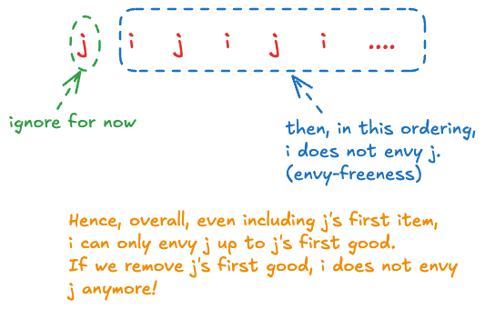
* **Envy-freeness up to one good (EF1)**: It’s a relaxation of envy-freeness so that each player may envy another player but only up to a single item, i.e., player $$i$$ may envy player $$j$$, but the envy can be eliminated by removing a good from $$j$$’s bundle. Formally, for any $$i,j \in N$$, if $$A\_j \neq \phi$$, then there exists a $$g \in A\_j$$ such that $$v\_i(A\_i) \geq v\_i(A\_j \setminus {g})$$. Notice that this $$g$$ can be different for different players (even for a fixed $$j$$)!

## Round Robin Algorithm

The good news is that we can satisfy EF1 by the round-robin algorithm. Let the players take tunrs choosing their favorite good from the remaining goods, in the order $$1, 2, \cdots, n, 1, 2, \cdots, n , 1, 2, \cdots$$ until the goods run out.

This works for any number of agents, and for any additive valuation functions.

The proof is actually really simple:

* If $$i$$ is ahead of $$j$$ in the round robin ordering, then in every round, $$i$$ does not envy $$j$$ (because $$i$$ would pick the good that she values more, because $$i$$ had the first choice) — envy-freeness.
* If $$i$$ is behind $$j$$ in the ordering, then consider the first round to start with $$i$$’s first pick (i.e., for now, ignore $$j$$’s first pick). Then, we can pretend as if $$i$$ is ahead of $$j$$ in all these rounds (if we’re ignoring $$j$$’s first pick, then we act as if $$i$$ picked frist). So, $$i$$ does not envy $$j$$ up to $$j$$’s first good. It’s possible that $$i$$ envies $$j$$ but that’s only because of $$j$$’s first good.&#x20;

<figure><img src="https://2994438412-files.gitbook.io/~/files/v0/b/gitbook-x-prod.appspot.com/o/spaces%2FixDr0QrEmvZAtfJXNbfW%2Fuploads%2F30JNmxipzvU2UzvraOfP%2Fimage%201.png?alt=media" alt=""><figcaption></figcaption></figure>

As a bonus, the resuting allocation is balanced: that is, the difference in the *number* of goods is at most 1, between any pair of agents.

## Envy-Cycle Elimination Algorithm

Note: this mechanism works for general monotonic (not necessarily additive!) valuations: $$v\_i(S) \leq v\_i(T)$$ for any $$S \subseteq T \subseteq G$$.

We can still get an EF1 allocation (even for a general monotonic valuation function) using this envy-cycle elimination algorithm:

1. Allocate one good at a time in an arbitrary order.
2. Maintain an envy graph with the players as its vertices, and a directed edge $$i \to j$$ if $$i$$ envies $$j$$ with respect to the current partial allocation.
3. At each step, the enxt good is allocated to a player with no incoming edge. Any cycle that arises is eliminated by giving $$j$$’s bundle to $$i$$ for every $$i \to j$$ in the cycle.

The key intuition here is this:

* If no one envies player $$i$$, then giving 1 good to player $$i$$ can only make players envy $$i$$ up to at most 1 good in the worst case.
* When we have a cycle, it’s an indication that we can make everyone happier by rotating the bundles along the cycle — since it makes every player strictly better off. So, the total utility strictly increases. (Hence, we can’t have infinite cycles, because the total utility of allocating finitely many goods must be finite.)

We prove the correctness of this algorithm (and the fact that it terminates) with the following 3 claims:

1. Claim 1: At each step, the procedure of eliminating cycles must end.
   * Each time we eliminate a cycle, we do so by cycling the bundles around so that the new allocation has strictly higher utility. So, the utilitaria welfare strictly increases, because everyone on the cycle gets strictly higher utility.
   * So, it cannot happen infinitely since the allocation has finite goods and must generate finite utility.
2. Claim 2: When the procedure of eliminating cycles ends, there is an unenvied player (i.e., a “source” in the envy-graph)
   * Proof by contradiction: Suppose not. Then, player a is envied by b, b is envied by c, and so on.. But we only have finitely many players. So, we end up with a cycle in the envy graph, which contradicts the fact that we removed all the cycles.
3. Claim 3: At each step, the partial allocation is EF1.
   * We only allocate a good to an unenvied player, so any envy towards that player is by at most one good (i.e., the newly allocated good)

Claims 1 and 2 are enough to prove the termination of the algorithm, while claim 3 is required to prove the correctness (since it states that at every step, the allocation is EF1, and so, even at the end, the allocation is EF1).

Notice that we don’t use the “additive”-ness at all! But we do use monotonicity (i.e., when we add a good to a player’s bundle, her valuation cannot decrease — she cannot start to envy others as a result of this allocation!)

## Maximum Nash Welfare (MNW)

MNW requires additivity of the valuation functions.

The Nash Welfare of an allocation is the product of the players’ utilities: $$\prod\_{i=1}^n v\_i(A\_i)$$.

{% hint style="warning" %}
**Theorem: An allocation that maximizes the Nash Welfare, called a Maximum Nash Welfare (MNW) allocation, is EF1.**
{% endhint %}

It’s a bit surprising that nash welfare (and not egalitarian welfare) leads to EF1 allocations.

Corner case: If MNW = 0, maximize the number of pllayers with positive utility first, and then maximize the Nash welfare among these players. This is the way to guarantee that the allocation satisifes EF1.

Proof sketch:

* Suppose for contradiction that playuer $$i$$ envies player $$j$$ even after removing any good from $$j$$’s bundle.
* Consider a good $$g$$ in $$j$$’s bundle that minimizes the ratio $$v\_j(g)/v\_i(g)$$ — that is, pick the good $$g$$ such that $$j$$ does not value it much, but $$i$$ does.
* Then, moving $$g$$ to $$i$$’s bundle can be shown to increase the Nash welfare.

Bonus: The resulting allocation is always **Pareto optimal**: we cannot make some player better off without making another player worse off. This is almost by definition because if we could, then we would do so and the Nash welfare (product of everyone’s utilities) will strictly increase (and the original allocation wouldn’t be “maximum” Nash welfare).

***

Quick Summary:

* All of Round-Robin, Envy-ycle Elimination, and MNW guarantee EF1
* Round-Robin ensures that the allocation is balanced.
* Envy-cycle does not require that the valuations are additive, only monotonic.
* MNW guarantees Pareto-optimality too.

So, each of them have their distinct advantage and hence, use-case.

## EFX

Recall that EF1 means “if a particular good $$g$$ is removed from your bundle, I will no longer envy you”.

Envy-freeness up to any good (EFX) states: For any $$i, j \in N$$ and ANY $$g \in A\_j$$, we have $$v\_i(A\_i) \geq v\_i(A\_j \setminus {g})$$. That is, “if ANY good is removed from your bundle, I will no longer envy you.”

Clearly, EFX is a stronger constraint than EF1.

In general, we have: Envy-freeness $$\implies$$ EFX $$\implies$$ EF1.

**The output of round robin, envy-cycle elimination, and MNW may NOT satisfy EFX.**

Wait.. does there always exist an EFX allocation in the first place??

For $$n = 2$$ and $$n = 3$$, yes, an EFX allocation always exists. The proof for $$n=2$$ is simple, while proof for $$n=3$$ is much more complicated.

Proof for $$n=2$$: Cut-and-choose algorithm

* The first player divides the goods into 2 bundles that are equal as possible in her view.
* Then the second player chooses the bundle tha the prefers.
* The first player will be EFX, and the second player will be envy-free.
  * The proof that the first player will be EFX relies on the fact that she divided the goods into 2 “as equal as possible” bundles.
  * Let $$d=v\_1(A\_2)-v\_1(A\_1) > 0$$.
  * Every object $$g$$ in $$A\_2$$ must have $$v\_1(g) \geq d$$ because otherwise player 1 would’ve moved $$g$$to the other bundle to make the bundles “more equal”.
  * So, removing any object $$g$$ from $$A\_2$$ will result in $$v\_1(A\_2 \setminus {g}) \leq v\_1(A\_2) - d = v\_1(A\_1)$$, and hence player 1 is EFX.

**For n** $$\geq 4$$**, this question is open! (there is neither an existence proof nor an impossibility result yet).**

## Maximin Share (MMS)

Until now, we had been relaxing the constraints of envy-freeness, and we saw that it’s always possible to obtain an EF1 allocation (and we saw multilpe different ways to achieve this, with additional properties of each algorithm).

Now, we hope to relax the proportionality condition (and one such relaxation yields the maximin share value).

A player’s maximin share (MMS) can be computed by performing the following thought experiment: The player divides the goods into $$n$$ bundles so as to maximize the value of the minimum-value bundle, and the value of the minimum bundle in such a partition is called the player’s MMS.

So, MMS means that each player thinks they’re getting *at least* the worst bundle in a “fair” allocation. Getting less than MMS would make the player doubt whether the allocation was fair (because in her head, she’s getting even less than the worst possible outcome assuming the goods are split so that everyone gets nearly equal value).

Note that maximin share is a relaxation of proportionality, i.e., $$MMS\_i \leq \frac 1 n v\_i(G)$$. The proof by contradiction is quite simple: suppose not, then each bundle in this MMS allocation has value strictly greater than $$\frac 1 n v\_i(G)$$, and so the sum of the valuations (using additivity of player $$i$$’s valuations) of each bundle gives: (total value) $$> n \cdot MMS\_i > v\_i(G)$$, which is not possible, since player i’s total value of $$G$$ should be the same, no matter the allocation. Basically, the lowest bundle’s value cannot be strictly greater than the arithmetic mean (which would be obtained when player i can divide all goods exactly equally).

An allocation that gives every player his / her maximin share always exists when there are 2 people, but NOT when there are at least 3 players (known impossibility proof). This shows how hard it is to satisfy MMS (let alone proportionality).

**However, for any number of players, we can always give every player more than** $$\frac 3 4$$ **of his / her maximin share.**

The proof that an allocation that gives every player at least his / her maximin share always exists when there are 2 players uses the cut-and-choose algorithm again:

* Alice divides the goods into 2 parts that are of as equal value as possible in her view.
* Either part yields value at least Alice’s MMS to her (by definition)
* Bob chooses a part that he prefers
* Bob is envy-free (and therefore, proportional, and therefore he gets his MMS). Recall that for 2 players, envy-freeness $$\equiv$$ proportionality and also, in general, proportionality $$\implies$$MMS.

(There’s also such a thing as minimax share — read up about it if you’re interested!)

## Query Complexity

It’s a way of comapring how complex different algorithms are. Sort of like the idea of time complexity.

With each query, the algorithm can find out a certain player’s value for a certain set of goods.

Then, the question is: how many tiems do we need to query the players? (How many times do we have to ask “oh hey Bob umm how much do you value this set of goods?”)

This becomes especially relevant when valuations are not additive — because in the worst case, we might have to make $$n2^m$$ queries.

BUT, thankfully, we don’t!

The envy-cycle elimination algorithm can be implemented using $$O(nm)$$ queries, even with monotonic (non-additive) valuations:

* It suffices to query the value of each agent for the $$n$$ bundles in each partial allocation to construct the envy graph.
* Since there are $$m$$ partial allocations, the number of queries is $$O(nm)$$

In each iteration, we add an item to an existing bundle — all other bundles remain unchanged. So, we only need to query the players’ valuations for this new bundle. And even during the cycle-elimination phase, the bundles just move around, they don’t actually change. So, the valuations each player has for the bundles don’t change, and we don’t have to re-query them. (We assume that we store the query results each time we get them).

In fact, if we have just 2 agents with monotonic valuations, $$O(\log m)$$ queries suffice (even though the total possible allocations is $$2^m$$ wow!). Proof:

* Arrange the goods on a line, and implement cut-and-choose
* The first agent can find an EF1 cut using binary search

The same technique does NOT work for EFX (even though an EFX for $$n=2$$ does exist, it cannot be found this way), as there may not exist an EFX partition on this specific arrangement of items on the line. e.g. if we have 3 goods, 2 players with identical and additive valuations 1, 2, 1 → there’s no way to make it EFX if we arrange them in the order 1, 2, 1 (we’d have to do 1 1 2 or 2 1 1).

In fact, any deterministic EF1 algorithm needs $$\Omega (\log m)$$ queries. That is, this $$\log m$$ bound is tight, and hence, we can write it as $$\Theta(\log m)$$ .

Proof:

* We will prove that *even* for identical additive valuations where each player has value 1 for 2 goods, and 0 for the rest, we need $$\Omega(\log m)$$ queries. (And here, the mechanism *knows* that both players have such valuations — 1 for 2 fixed goods (e.g. gold coins), and 0 for the rest (e.g. stones)) And hence, we need at least these many queries for a more general case, since in general, the mechanism doesn’t know the player’s valuations apriori without querying!
* Notice that in ANY EF1 allocation, the two valuable goods (with valuation = 1 each) must be separated. So, the goal of the mechanism is to create a partition such that each bundle contains 1 of the valuable good.
* We can show that such a mechanism would require $$\Omega(\log m)$$ queries by making use of an adversary argument → assume an adversary whose job is to respond to the queries so that the mechanism takes the maximum number of querie (i.e., the adversary makes life difficult for the mechanism).
* In particular, as the adversary that generates that testcase, we don’t have to decide apriori what the valuable goods are, as long as our answers to the queries are consistent to what we finally declare the valuable goods to be! The mechanism only sees the query results, and only finds out the valuations at the very end (to make sure we weren’t cheating)
* Let $$G'=G$$ initially (the mechanism needs to find a way to split the two valuable goods, so we wil play the role of the adversary and track which set contains both the valuable goods in our head).
* Suppose the algorithm queries $$v(H)$$.
* If $$|G' \cap H| \geq \frac{|G'|}{2}$$, then we answer 2 and replace $$G'$$ by $$G' \cap H$$. That is, okay, we told the mechanism that both valuable goods are in $$H$$, and previously we had told the mechanism that they are in $$G'$$ → hence, to be consistent, they must be in $$G' \cap H$$ now — but we only do this when the set containing both is bigger than the set not containing both, and that’s exactly what we want → we want to force the set containing both the valuable goods to be as large as possible.
* Otherwise, we (the adversary) answer 0 and replace $$G'$$ by $$G' \setminus H$$. (obviously we never want to answer 1 if we can avoid it, otherwise the mechanism can simply output $$H,G \setminus H$$ as the two partitions and its done)
* Since $$|G'| =m$$ at the beginning, and decreases by a factor of at most 2 after each query, at least $$\log\_2 m$$ queries are needed to “split” the two valuable goods, in this worst case.
* Hence, any deterministic EF1 algorithm needs $$\Omega(\log m)$$ queries.

{% hint style="info" %}
Any deterministic EFX algorithm needs a number of queries **exponential** in $$m$$ (not just linear, but exponential! Much much harder than EF1)
{% endhint %}


# Cake Cutting

Last week, we dealt with the problem of trying to fairly divide a set of indisivible goods.

Now, we’re trying to divide a heterogeneous divisible good among interested agents with different preferences.

Here, hetereogeneous means that agents have different preferences for different parts of the good. It’s useful to imagine a slice of cake (from left to right), and agents have different valuation functions throughout the cake.

The cake could represent land (some agents value some parts of the land more than others), machine processing time (some agents may want to use the machine in the morning, others in the afternoon, etc.)

The key thing to note here is that we can always divide the cake into smaller pieces — so, it’s a continuous space, rather than the discrete goods we’ve been dealing with so far.

## Setting

* The cake is represented by the interval $$\[0, 1]$$
* Set of agents $$N = {1, 2, \cdots, N}$$
* Agents have valuation functions $$v\_1, \cdots, v\_n$$ over the cake.
* The valuation functions are:
  * Non-negative: There is no bad piece of cake — you would never be worse off if you’re given some additional piece of cake, no matter which part.
  * Additive: Values of disjoint pieces of cakes add up — there is no interaction effect between different pieces of the cake
  * Nonatomic: The value of any single point is 0 — e.g. we don’t allow a cherry that cannot be cut, since that would bring us back to the “indisivible” problem domain
  * Normalized: The value of the whole cake is 1, for each agent — this assumption can be made without loss of generality because we can always scale / normalize the valuation functions. We do this so that the valuations across agents are comparable.
* Allocation $$A = (A\_1, \cdots, A\_n)$$
* Each $$A\_i$$ is a union of finitely many intervals. The allocation $$A$$ is “connected” if each $$A\_i$$ is a single interval — that is, each agent only gets a single (connected) slice of cake, and not multiple disjoint slices.

### Valuation Functions

For convenience, we write $$v\_i(x, y)$$ instead of $$v\_i(\[x,y])$$ to denote agent $$i$$’s valuation for the interval $$\[x,y]$$ of cake, where $$0 \leq x \leq y \leq 1$$.

The valuation function $$v\_i$$ is often specified through the density function $$f\_i$$ where:

* $$v\_i(B) = \int\_B f\_i(x) dx$$ for $$B \subseteq\[0,1]$$ — that is, we can integrate $$f\_i$$ over the cake’s interval to get agent $$i$$’s valuation for that interval.
* Normalization: $$\int\_0^1 f\_i(x)dx = 1$$ — visually, this means that the area under the curve of $$f$$ in the interval $$\[0,1]$$ is exactly 1.
* And then we get additivity and non-atomicity “for free” simply by the properties of integration.

## Fairness Notions

And as always, we’re interested in allocations that are “fair”, and so we need to define what that means.

We can use the same notions from last lecture with indivisible goods:

* Proportionality: $$v\_i(A\_i) \geq \frac 1 n$$ for all $$i \in N$$
* Envy-freeness: $$v\_i(A\_i) \geq v\_i(A\_j)$$ for all $$i, j \in N$$ → means that i would not want to have any other agent’s cake instead of my own.

For $$n=2$$, envy-freeness and proportionality are equivalent.

For $$n \geq 3$$, envy-freeness is strictly stronger than proportionality (since it is not only concerned with how much cake you got compared to the whole cake, but you’re also concerned about how the rest of the cake got allocated among the other agents, i.e., you not only care about your own piece of cake, but also everyone else’s piece of cake).

## Two Agents: Cut-and-Choose

Note that the cut-and-choose protocol is always meant only for 2 agents. So, whenever we say cut-and-choose, we’re implicitly assuming there are only 2 agents.

Agent 1 cuts the cake into two (exactly!) equal pieces, according to her opinion. And this is possible because the cake is divisible — note that previously we could not do this, and so we had to say “divide the goods into 2 sets that are as close as possible to each other in value”.

Agent 2 then chooses the piece that he prefers.

Agent 2 is clearly envy-free since he picked the piece, and agent 1 is envy-free because he cut the cake such that both pieces were exactly equal in the first place.

So, this allocation is envy-free (and hence, proportional too).

## Robertson-Webb Model

Cut-and-choose is clearly a “simple” protocol. But how do we quantify how simple it is.

Basically, we’re trying to come up with a way to quantify the complexity of an algorithm like how we did for divisible goods, by making a notion of “query complexity”.

We do nearly the same thing here, using the Robertson-Webb model.

Under this model, our algorithm can only make two types of queries:

* $$Eval\_i(x, y)$$ → returns $$v\_i(x, y)$$ — the value of agent $$i$$ for the interval $$\[x, y]$$
* $$Cut\_i(x, \alpha)$$ -. returns the leftmost point $$y$$ such that $$v\_i(x, y) = \alpha$$, or states that no such point exists.

Then, for cut-and-choose, we only need to perform 2 Robertson-Webb queries:

* The cutter needs to query $$Cut\_1(0, 0.5)$$ and then we get some output $$k$$
* And then the chooser queries $$Eval\_2(0, k)$$ to decide whether he prefers the first piece or the second piece (which will have value $$1-$$ (the value of the first piece), so we don’t have to query again.

## Dubins-Spanier Protocol

Achieves proportionality for any number of agents. Notice that this wasn’t even possible in the case of indivisible goods.

Algorithm:

* A referee moves a knife over the cake starting from the left
* Repeat until there is only 1 agent left:
  * When the piece of cake to the left of the knife is worth $$\frac 1 n$$ to some agent, that agent shouts “stop!” and leaves the procedure with that piece of cake.
* The last agent gets the remaining cake.

Btw this algorithm is non-truthful in that players can gain more utility by misreporting — intuitively, if i know that you value only the right half of the cake (uniformly) and i value the entire cake uniformly, i can take 3/4 of the cake before yelling stop; so i get value 3/4 by shouting stop later, and you get value 1/2.

Proof of proportionality: If a player shouts “stop” and gets a piece of cake, he gets (what he thinks is) at least $$\frac 1 n$$ of the cake, so anyone who shouts stop satisfies proportionality. Now, the remaining people did not shout stop — so they think that piece of cake was worth $$\leq \frac 1 n$$ and so the remaining cake must be worth $$\geq \frac{n-1}{n}$$, to be split among $$n-1$$ people (so it’s still possible for everyone to get a proportional share). And we can use inductive logic here, till there are only 2 people, and the last person will also think that he gets $$\geq \frac 1 n$$. Basically, in every round, those who did not yell “stop” think that the remaining cake has enough for everyone else to get a proportional share — and this invariant is true in each round, until the very end.

In fact, every agent gets exactly value $$\frac 1 n$$ and the last agent gets *at least* $$\frac 1 n$$.

How many Robertson-Webb queries do we need to implement this protocol? $$O(n^2)$$ queries. Don’t think of the algorithm in terms of moving a knife anymore — think of how you would implement using Cut and Eval queries.

Because in each round, we need to ask all the remaining agents their value for $$Cut\_i(k, \frac 1 n$$) where $$k$$ was the cut-point in the previous round (in round 1, $$k=0$$). And then the algorithm gives the cake to the agent with the lowest value of $$Cut\_i(k, \frac 1 n)$$ becuase he would have shouted “stop” first when the knife reached that point. And then we repeat this for $$n-1$$ rounds in the worst case, so we have the number of queries be: $$n + (n-1) + \cdots + 2 = O(n^2)$$

## Even-Paz Protocol

Achieves proportionality for any number of agents, *with fewer queries*.

Assume for simplicit that $$n$$ is a power of 2 (this is only to make the analysis simpler, but doesn’t actually affect the algorithm).

The idea is to use divide-and-conquer. Instead of Dubins-Spanier, which only reduces the number of players by 1 in each round, we hope to split the agents into 2 groups in each round — one that values the left half more, and the rest who value the right half more. More precisely:

1. Each agent marks the point that divides the cake into two halves of equal value, according to his / her own opinion.
2. Let $$t$$ be mark number $$n/2$$ (median-ish) from the left.
3. Recurse on $$\[0, t]$$ with the left $$n/2$$ agents and on $$\[t, 1]$$ with the right $$n/2$$ agents.
4. Base case: When we’re down to one agent, that agent gets the whole cake.

It’s very similar to merge-sort / quicksort with median pivot.

The number of queries is clearly: $$Q(n) = 2Q(n/2) + O(n)$$, which yields $$Q(n) = \Theta(n \log n)$$.

In each round, each agent submits their $$Cut\_i(0, 0.5)$$ values to the algorithm. And then once the algorithm determines the pivot (about which it will recurse), then it asks for each agent’s $$Eval\_i$$ values, depending on whether they’re in the left-set or the right-set (we can technically achieve proportionality even if we don’t call $$Eval\_i$$ for all agents, but in Even-Paz, we do this because we need to *recurse*, which means they need to know how much they value this part of the cake). So, we do $$2n$$ queries per round. And we can draw the recursion tree which has height $$\log\_2 n$$, and each level has cost $$2n$$. So, the total cost is $$\Theta(n \log n)$$

Actually, we can pick any point to the be “pivot” here, not just the median point (assuming we ask the agents to report the corresponding cut value), and the algorithm will still be correct in that all players will get their proportional share. In fact, if we always pick the first (left-most) point to be the pivot (when we've asked all of them to report how much of the cake is worth 1/n to them), then this reduces to Dubins-Spanier algorithm, since in each round, the person with the left-most cut gets the cake! We use median to get the query complexity down to $$n \log n$$ but we could’ve also used any other (constant) fraction instead of $$\frac 1 2$$, e.g. even if we split the cake $$\frac 1 3 : \frac 2 3$$, we would still get a $$n \log n$$ query complexity.

The proof of proportionality is very similar to Dubins-Spanier — in each round, the left-set agents think that their side of the cake is worth more than the right side so they got the better end of the bargain, and vice-versa for the right-set. Each group of players is happy to be in whichever group they’re in, because they think there’s enough cake to be divided among the players in that group. And this holds true during each recursive step, so it holds true even when we reach the base-case of a single player. So, each player gets at least their proportional share.

Implementation detail: If we’re left with two agents, and we recurse on the left-half first, then the left agent gets *exactly* their proportional share, and the right agent gets *at least* their proportional share.

<figure><img src="https://2994438412-files.gitbook.io/~/files/v0/b/gitbook-x-prod.appspot.com/o/spaces%2FixDr0QrEmvZAtfJXNbfW%2Fuploads%2FDV2vqPM0qPnek45qks6J%2FScreenshot_2024%2010%2024_at_8.43.48_AM.png?alt=media" alt=""><figcaption><p>Example run of Even-Paz. Notice that red and yellow get exactly what they think is a quarter of the cake, whereas blue and green get more than their quarter. Also notice that the order of yellow and green cuts swaps from round 1 to round 2 — this is possible (e.g. green might have valued the left half of the cake more than yellow, but with that removed, green’s new “midpoint” for the right half goes much further right).</p></figcaption></figure>

{% hint style="warning" %}
$$O(n \log n)$$ **is the optimal number of queries among ALL proportional protocols,&#x20;*****even if the allocation is not required to be connected*****.**
{% endhint %}

And Even-Paz guarantees connected pieces too, so it’s really amazing!

## Envy-Freeness

So far, we’ve discussed envy-freeness for 2 agents (using cut-and-choose) and proportionality for any number of agents (Dubins-Spanier and Even-Paz).

Now, we discuss envy-freeness for 3 agents.

Firstly, such an allocation is possible, and is achieved by the Selfridge-Conway protocol. It takes 5 cuts and 9 queries (not worth getting into *how* it’s done).

The key point is that envy-freeness is MUCH harder than proportionality because each agent cares about everyone else’s pieces too.

Aziz and Mackenzie (2016) proposed the first bounded envy-free protocol for any number of agents, with the bound being $$n^{n^{n^{n^{n^n}}}}$$for both, the number of cuts and queries. So, it’s “bounded” but really only for theoretical interest.

The current best lower bound on the number of cuts and queries is $$\Omega(n^2)$$.

### Envy-Freeness Approximation

And so, even though envy-freeness is always possible to achieve, it might be too slow in many cases.

Luckily, we have an approximation algorithm in which any agent envies any other agent by at most $$\frac 1 3$$. Note that this envy can be considered really huge if we have like $$n=100$$, and each person is supposed to get only $$\frac 1 {100}$$ (and so the relative envy is a lot).

Algorithm (variant of Dubins-Spanier):

1. The referee moves a knife over the cake starting from the left.
2. When the piece of cake to the left of the knife is worth $$\frac 1 3$$ to some agent, that agent shouts “stop”, and leaves the procedure with that piece. (Note that this remains $$\frac 1 3$$ *no matter* how many agents we have!)
3. Suppose the knife reaches the right end of the cake, but some cake is still unallocated:
   1. Case 1: There are still agents left. The remaining cake is given to one of them arbitrarily.
   2. Case 2: There is no agent left. The remaining cake is given to the agent who received the last piece (to ensure connectivity).

Proof that any agent envies another by at most $$\frac 1 3$$:

* Consider an agent that shouts stop, and gets a piece at any step. That agent gets value $$\frac 1 3$$. So, the remaining cake must be worth $$\frac 2 3$$ to this agent. So, in the worst-case, even if the entire remaining cake goes to some other agent, the envy will be at most $$\frac 2 3 - \frac 1 3 = \frac 1 3$$.
* Consider an agent $$i$$ that does not get any cake. In each round, he did not shout stop before any other agent. So, $$i$$’s value for the cake that any other agent gets is at most $$\frac 1 3$$. So, his envy towards any other agent can be at most $$\frac 1 3$$.

In fact, using this approach, $$\frac 1 3$$ is the best we can do (i.e., we’ve chosen this number carefully — because we need to balance the envy in both cases, to minimize the maximum envy. It’s not that hard to see why (think what would happen if we used $$\frac 1 5$$ instead of $$\frac 1 3$$ in step 2).

## Truthfulness

Is the cut-and-choose protocol truthful? No for the cutter, yes for the chooser. Obviously if you know the chooser’s valuation, you can try to abuse that so that you get more than 0.5 of the cake. But as the chooser, you literally just get the piece you pick so you have no incentive to lie.

In fact, none of the mechanisms we’ve seen so far (Dubins-Spanier, or Even-Paz) are truthful for all players — i.e., at least one player has an incentive to lie under some conditions. Hence, the algorithms are not truthful.

Note that whenever we talk about “truthful”, we’re asking “is there ANY possibility that lying is better?” (including the case in which you know your opponent’s valuation / strategy / anything!)

There is a pretty cool / simple truthful mechanism for when ALL agents have a piecewise uniform valuation, i.e., for each agent $$i$$, the density function takes on the values only 0 or some $$s\_i$$. Different agents can have different values for $$s\_i$$ (that’s why it depends on $$i$$) but each agent can only have 1 non-zero value for $$s\_i$$.

<figure><img src="https://2994438412-files.gitbook.io/~/files/v0/b/gitbook-x-prod.appspot.com/o/spaces%2FixDr0QrEmvZAtfJXNbfW%2Fuploads%2FWwvszoiP6a39dcn1yj1U%2Fimage%202.png?alt=media" alt=""><figcaption></figcaption></figure>

The algorithm works as follows:

* Agent 1 starts at the left end of the cake, and agent 2 at the right end
* Each agent eats her desired part of the cake at the same speed until they meet. Here, meet is defined as “agent 1 crosses agent 2 on the x-axis, even if it is mid-air when either one is jumping forward”
* Any part that an agent jumps over goes to the other agent immediately. (And the other agent can eat this later, after the algorithm ends)

Basically what the piecewise uniform constraint means is that each agent either doesn’t like the part or it likes it (equally as all other parts it likes). Among the parts it likes, it has no preference for some parts over another. The reason we need this is so that you have no incentive to skip eating a piece you like to move faster towards a piece you like even more — these means that when you’re at a piece you like, you should just eat that piece because you’ll be getting the same amount of utility per unit eating time, and by jumping forward, you will have lesser total time to eat (because you’re going to meet the opponent sooner).

All the time you spend is only to eat the cake (you can teleport to the piece you want to eat instantly), and you both eat at the same speed. So, you have no reason to envy the other player — because you both spend the same amount of time eating, so the amount of value you get (by eating your piece) must be the same (or more) as the value you get if you had eaten the other agent’s intervals of cake (it’s more when he skips some cake that you value, so you get that directly)

Example of the cake-eating algorithm:

<figure><img src="https://2994438412-files.gitbook.io/~/files/v0/b/gitbook-x-prod.appspot.com/o/spaces%2FixDr0QrEmvZAtfJXNbfW%2Fuploads%2FKHVrwnRnlNM7A81wqGTw%2FScreenshot_2024%2010%2024_at_12.36.21_PM.png?alt=media" alt=""><figcaption></figcaption></figure>

Rough Proof of truthfulness:

* I won’t say i like a piece of cake if I don’t actually like it → because it does not give me any value by eating it, and I’m wasting time eating useless cake
* I won’t skip over any cake that I like → because my valuation function is piecewise uniform, even if i jump to a part, i would like that part equally as much as i like this one. So, i might as well eat what i like now instead of skipping it for later.

Even for a piecewise constant function (i.e., each agent’s valuation for any interval is a constant value), this algorithm does not work. In fact, there cannot be any envy-free truthful mechanism *even with piecewise constant functions with 2 agents*.

This show hows hard (read: impossible) it is to satisfy envy-freeness and truthfulness in the general case.


# Rent Division

## Setting

We want to faily distribute rooms and rents amongst roommates.

* Roommates (players): $$N = {1, \cdots, n }$$
* $$r$$ : rent price for the whole apartment
* $$v\_{ij}$$ ; player $$i$$’s value for room $$j$$ such that $$\sum\_j v\_j = r$$
  * The sum of the rents across all rooms must be equal to the rent of the apartment, otherwise you don’t think the apartment is worth it (and if your value is more, you’lll end up paying more per room, so. you should just scale everything down to reach a sum of $$r$$)

And then, siimlar to auctions, our mechanism needs to determine 2 things:

* Who gets what? In this case, a room allocation $$\sigma : N \to N$$, i.e., each player should be assigned a room.
* Who pays what? Rent division $$\vec p = p\_1, \cdots, p\_n$$ such that $$\sum\_j p\_j = r$$ where $$p\_j$$ is rent for room $$j$$ (and so, the player assigned to room $$j$$ must pay $$j$$).

Note that we can’t just auction off the rooms one by one, because then players might not be truthful, and it might not lead to an envy-free allocation (and it wouldn’t even maximize utility).

Also, note that the requirement that $$\sum\_j v\_{ij} = r$$ means that players can’t encode views such as “I prefer room 1, but can’t afford to pay more than $500 for it”. And it also does not take into account that some players might have more disposable income than others, i.e,. some might be willing to pay more for their favorite rooms such that $$\sum\_j v\_{ij} > r$$ (but this is not allowed).

## Envy-Free Outcome

In this context of rent division, the definition of envy-free is basically the same, but it needs to take into account the price that each person is paying. That is, each player should think “I do not prefer your room for the price you’re being charged, to my room for the price i’m being charged.”

Another easier way to look at it is that: you would not want to change your position for anyone else’s position (which is what envy-free means even in english).

More concretely, if the outcome is $$<\sigma, \vec p>$$ then, for all $$i, j \in N$$, we must have: $$v\_{i \sigma(i)} - p\_{\sigma(i)} \geq v\_{ij} - p\_j$$. Note that we assume players have a quasilinear utility function (i.e., getting $x gives you the same marginal utility no matter how much money you currently have).

## EF Allocation

It’s natural to ask: does an EF allocation even exist??

And it turns out that the answer is YES, and can be efficiently computed. But such an EF allocation is not unique.

In fact, this algorithm is an example of a provably fair solution — this means that given the outcome, if anyone objects, you can easily prove / convince him that he’s wrong (in an economic sense, he wouldn’t be better off swapping places with anyone else).

Also, this mechanism guarantees efficiency in the economic sense (Pareto optimality) — it is impossible to find another assignment of rooms to players that benefits a roommate without making another player worse off.

The general framework for coming up with an EF allocation is a 2 step procedure:

1. Deciding who gets what, i.e., room assignment

   Compute a socially optimal allocation of players to rooms, by using weighted-MCBM (Maximum Cardinality Bipartite Matching) ← this step that can have multiple room assignments that all yield the same social welfare.
2. Decide who pays what, i.e,. rent division.

   Find an EF price vector using linear programming — you have a set of constraints and you want to maximize a function

Both weighted-MCBM and LP can be solved in polynomial time.

## Beyond EF

But… in some cases, even EF is not enough (pun intended). What we mean by this is that EF is not enough to for the division to feel “fair”. So, we want to capture some other notions of fairness too.

Consider the following example:

<figure><img src="https://2994438412-files.gitbook.io/~/files/v0/b/gitbook-x-prod.appspot.com/o/spaces%2FixDr0QrEmvZAtfJXNbfW%2Fuploads%2FnJ1ZuR2ItFX36FE1K39j%2FScreenshot_2024%2010%2028_at_6.00.55_PM.png?alt=media" alt=""><figcaption></figcaption></figure>

It’s pretty clear who gets what, but what if Alice pays the entire rent of $3000? This is still envy-free (since Alice wouldn't envy anyone because she has value = 0 for the other two rooms, and of course, Bob and Claire are more than happy with this since they don't have to pay for anything). But… it still feels like Bob and Claire are much happier than Alice in this scenario (both of them have utility = 2000, and Alice has utility = 0).

Note that at this point, the rooms have already been allocated, and we’re only trying to play around with how much rent each person pays to make it as “even” as possible.

So, we want the players’ utilities to be “close to each other”, while also satisfying EF (of course, we don’t want to lose the very nice EF property — we’re trying to make it even stronger). There are two similar ways we can quantify this:

* Equitability (under EF constraint): Define $$D(\vec p) = \max\_{i, j \in N} (u\_i (\vec p) - u\_j (\vec p))$$ to be the maximum difference in the utilities of any 2 players under the rent division $$\vec p$$. Then, we’re trying to find $$\vec p$$ to minimize $$D(\vec p)$$ such that $$\vec p$$ is EF. This is sort of trying to distribute the utility as equitably as possible.
* Maximin (under EF constraint): Basically egalitarian, trying to maximize the minimum utility of any player. Formally, $$U(\vec p) = \min\_i u\_i (\vec p)$$ and then we’re trying to find $$\vec p$$ to maximize $$U(\vec p)$$ such that $$\vec p$$ is EF. So, the least happy person should be as happy as possible.

Luckily for us…

{% hint style="warning" %}
**Under EF-constraints, there is a unique maximin price vector, and it is also equitable**
{% endhint %}

which means that we don’t have to choose between the two notions of fairness — we can have both satisfied simultaneously!

However, note that there exists equitable price vectors that are not maximin. (For $$n=2$$, they are equivalent though).

And it turns out that humans do care about equitability / maximin in addition to just envy-freeness, as demonstrated by a study conducted by [spliddit.org](http://spliddit.org)


# Committee Voting

## Problem

Unlike auctions where everyone gets different things depending on what they want, in a voting setting, everyone gets the same thing (although they have different preferences). So, we’re trying to select a public outcome that is shared by everyone. e.g. everyone gets the same president.

In general, there are many different types of voting ballots (i.e., inputs):

* ranking → each voter submits an ordering for the candidates
* score → each voters submits a number for each candidate
* approval → each voter submits a subset of approved candidates
  * basically, each voter submits 1 for the candidates they approve, and 0 for the rest.
  * advantage: it’s simple and less cognitive effort is required from the voters’ perspectives (they just have to think whether or not they approve the voter, no relative comparisons needed);
  * disadvantage: it does not allow refined or combinatorial preferences (e.g. i can’t say “i want to approve A and B, but only if they are chosen together” or “i like A more than B”)

And there can be many different kinds of outputs of voting:

* single winner → e.g. president of a student council
* multiwinner / committee e.g. student council committee, dishes to serve in a reunion party. in this case, all the selected members of the committee are “equal” so the decision is just whether or not to include or exclude from the committee
* ranked committee → e.g. a committee consisting of president, vice-president and a secretary, where there’s some ordering in the positions of each member of the committee.

In this lecture, we’re only looking at approval voting in a multi-winner category

## Approval Committee Voting Setting

* Voters $$N = {1, \cdots, n}$$
* Candidates $$C$$, where $$|C| =m$$
* Voter $$i$$ approves a set of candidates $$A\_i \subseteq C$$
* We want to choose a committee $$W$$ of size $$k$$ where $$k \leq m$$ is given (that is, we don’t get to decide the size of the committee — $$k$$ is an input to our mechanism, not something we can control)
* Voter $$i$$’s utility is: $$u\_i(W) = |A\_i \cap W|$$, i.e., how many members of the selected committee did voter $$i$$ approve (which makes sense, because you feel happier if people you approve of are selected)

Note that the above definition of voter utility remains the same even when we consider any other metrics / scores to optimize.

Also, we can think of some natural metrics to evaluate how good a committee selection is:

* (Utilitarian) Social Welfare → total number of approvals obtained by members of the committee (i.e., “excellence”). Notice that this is the same as the total utility of all the voters, because we can swap the order of the sums.
* Coverage: number of voters who approve at least one committee member (”diversity”). This is “kind of” an egalitarian metric in that we’re trying to minimize the number of voters with zero utility, but we don’t distinguish between any non-zero values so it’s not *really* egalitarian.

Also, if a voter approves a candidate, we say that the candidate covers the voter (since picking this candidate is enough to make this voter have non-zero utility).

## Approval Voting (AV) and Chamberlin-Courant (CC)

Then, we can select committees trying to maximize these two metrics:

* Approval Voting (AV) → select a committee maximizing social welfare
* Chamberlin-Courant (CC) → select a committee maximizing coverage

Of course, there need not be a unique committee in each of these cases.

Moreover, AV is a truthful mechanism (since you’re trying to boost the number of votes your preferred candidates have) whereas CC is not (e.g. it’s possible to get more utility by reporting a truncated set of approved candidates).

## Beyond AV / CC

Consider this example:

* $$n = 301, m = 5, k = 3$$
* First 200 voters approve $${a, b, c }$$
* Next 100 voters approve $${d}$$
* And the last voter approves $${ e}$$

Then, AV chooses $${a, b, c}$$ and CC chooses $${a, d, e}$$.

But, neither feels “proportional” or fair. Because these committees don’t really reflect the “approval profile”.

A more proportional committee would be something like: $${a, b, d }$$ → since $$\frac 2 3$$ of the voters agree on $$a$$ and $$b$$, they should get $$\frac 2 3$$ of the seats on the committee, while only $$\frac 1 3$$ of the voters agree on $$d$$, so they should get $$\frac 1 3$$ of the seats.

Intuitively, a sufficiently large group of voters that agree on sufficiently many candidates should be correspondingly / proportionately represented / satisfied in the committee.

## Justified Representation

There are $$n$$ voters and $$k$$ committee slots, so a group of $$n/k$$ voters “deserves” one slot (of representation).

**First attempt**: For a group of voters $$S \subseteq N$$ such that $$|S| \geq \frac n k$$ and $$|\cap\_{i \in S} A\_i| \geq 1$$, we have $$|(\cap\_{i \in S} A\_i) \cap W| \geq 1$$. Basically, we’re saying that if we have a big enough group that together deserve at least one slot, and that they agree on at least one candidate, then at least one of the candidates they agree on should be selected in the committee.

This turns out to be too strong of a requirement, which cannot always be satisfied. For example:

* $$n=m=4, k = 2$$
* $$A\_1 = {a, b }, A\_2 = {b, c }, A\_3 = {c, d }, A\_4 = {a, d }$$
* Then, if we apply the rule above, then we would be forced to include all of $$a, b, c, d$$, but this exceeds the committee size.

To make our vocabulary / notation simpler, let’s call a group of voters $$S \subseteq N$$ such that $$|S| \geq \frac n k$$ and $$|\cap\_{i \in S} A\_i| \geq 1$$ to be a **cohesive group**. Basically a cohesive group makes up for at least one-slot-worth of representation, and agrees on at least one candidate (if they don't agree, they aren't "cohesive" and we can't do much to please them anyway).

Then, a justified representation (JR) is any committee that satisfies the following property: for any cohesive group of voters $$S \subseteq N$$, there exists $$i \in S$$ such that $$|A\_i \cap W| \geq 1$$.

Basically, JR says that in any cohesive group, at least one voter should have non-zero utility. So, no cohesive group should go unrepresented. But It kind of feels… too weak? Since we only require *one* voter to feel happy (in fact, just non-zero happiness), *no matter how big the cohesive group is*.

Also, it’s easy to see that AV may fail JR. Consider $$n=k=3, m = 4$$ where the first 2 voters approve $$a,b,c$$ and the last voter approves $$d$$, then AV picks $$a,b,c$$ but then the last voter is a cohesive group and has zero utility, hence does not satisfy JR).

Claim: CC always satisfies JR. Proof:

* Suppose for contradiction that it does not.
* Then, let $$S$$ be a cohesive group of voters that is unrepresented by the CC committee $$W$$, and let $$x$$ can be a candidate approved by all voters in $$S$$.
* Consider the marginal contribution of each $$w \in W$$ to the coverage. This is the number of voters who approve $$w$$ but no one else in $$W$$.
* Since teh coverage of $$W$$ is $$< n$$, the marginal contribution of some $$w^\* \in W$$ is less than $$\frac n k$$ (otherwise, if everyone’s marginal contribution is at least $$\frac n k$$, then all voters should be covered).
* So, we can remove $$w^\*$$ and add $$x$$ to obtain a higher coverage, which contradicts the fact that $$W$$ is CC. So, any CC committee also satisfies JR.

Hence, JR can be satisfied for any $$n, k, m$$ and approval profile.

## GreedyCC

Computing a CC committee is NP-hard (can be shown via a simple reduction from SET-COVER).

Fortunately, there is a greedy variant that runs in polynomial time (of course this does not guarantee maximal coverage, but it’s not bad).

The GreedyCC algorithm is quite simple: In each step, choose a candidate that covers as many uncovered voters as possible (i.e,. ignore the voters that are already happy and focus on the ones you want to cover). Repeat this until $$k$$ candidates have been chosen.

We claim that GreedyCC satisfies JR, and the proof follows exactly as above (i.e., if not, then there must’ve been a candidate who covers $$\frac n k$$ voters but we didn’t pick him in favor of someone else who satisfies less than $$\frac n k$$voters; this can’t happen because of the greedy nature of our algorithm).

## Extended JR

But one can ask the same question as asked AV and CC to JR: is JR sufficient?

Consider this example: Suppose have 100 voters, and 20 candidates and $$k=10$$. The first 50 voters like the first 10 candidates, and the next 50 voters like the next 10 candidates. Then, intuitively, we want to pick 5 out of 10 candidates from each group to be “proportional”. But even picking 9 from group 1 (i.e., that the first 50 voters approve) and 1 from group 2 satisfies JR.

So, our requirement of JR is too weak! So, we use **Extended Justified Representation (EJR)**.

To explain what EJR means, let’s strengthen our notion of cohesive groups first.

For a positive integer $$t$$, call a group of voters $$S \subseteq N$$ such that $$|S| \geq t \cdot \frac n k$$ and $$|\cap\_{i ]in S} A\_i | \geq t$$ a $$t$$-cohesive group. (Then, the previous definition of cohesive group is simply when $$t=1$$.)

Also, note that a $$p$$-cohesive group is always an $$r$$-cohesive group for any $$r \leq p$$, i.e., increasing the “order” of the cohesive group just strengthens the requirement, which is clear from the definition.

Then, a committee is said to satisfy EJR when: for any positive integer $$t$$ and any $$t$$-cohesive group of voters $$S \subseteq N$$, *there exists* $$i \in S$$ such that $$|A\_i \cap W| \geq t$$.

Notice that we still require only one of the voters in $$S$$ to have a utility of at least $$t$$ (others might get utility = 0 and that’s fine).

(Well, not really, we can show that under EJR, in any $$t$$-cohesive group $$S$$, the average utility of each person is more than $$\frac{t-1}{2}$$, so this definition is actually quite strong, even if it doesn’t seem like it.)

And this fixes the problem with JR.

## Proportional Approving Voting (PAV)

Fix an infinite non-increasing sequence $$s\_1, s\_2, \cdots$$

Thiele methods: A family of methods that involve choosing a committee $$W$$ by maximizing the score: $$\sum\_{i \in N} (s\_1 + s\_2 + \cdots + s\_{u\_i(W)}$$.

So, basically this sequence $$s\_1, s\_2, \cdots$$ captures the utility function of the players. If a voter $$i$$ has $$p$$ of his approved candidates in the committee $$W$$, then his utility is $$s\_1 + \cdots + s\_k$$. In particular, the marginal utility to voter $$i$$ of the $$k$$th approved candidate being part of $$W$$ is $$s\_k$$.

(Note that this sequence is from the *mechanism's* point of view -- i.e., it is the mechanism's assumption of how the voter utility functions behave. BUT from the voter's point of view, the term "voter's utility" still just represents the number of approved candidates in the committee for any voter. To de-confuse, we can use "score" to represent a voter's sum $$s\_1 + \cdots + s\_k$$.)

This makes intuitive sense, because we want to capture the effect of diminishing marginal utility of the voters. Once you already have 5 approved candidates in $$W$$, then the 6th one cannot give you more (marginal) utility than the first one did. This is why the sequence needs to be non-increasing.

Notice that each voter has the same sequence — this is done to ensure that we treat all voters symmetrically, i.e., we don’t favor any voter over any other.

Then, AV is just a special case of this with $$s\_i = 1$$for all $$i$$. Even CC is just a special case of this with $$s\_1 = 1, s\_i = 0$$ for all $$i > 1$$.

In Proportional Approval Voting (PAV), we set: $$s\_i = \frac 1 i$$ for each $$i$$.

(So the utility function for each player follows a kind of $$\log$$ graph, since $$\int\_x \frac 1 x dx = \ln x$$)

This means that if a voter approves $$r$$ candidates in the committee, the voter contributes $$1 + \frac 1 2 + \cdots + \frac 1 r$$ to the score of the committee.

The number $$1 + \cdots + \frac 1 r$$ is the $$r$$th harmonic number, usually denoted by $$H\_r$$.

But… why harmonic numbers? Why does this work?

Because they result in a roughly proportional committee. The intuition is that AV is precisely utilitarian, CC is kind of egalitarian (up to a certain point), and PAV is kind of like Nash.

And the reason that PAV is like Nash is because maximizing $$\sum\_{i \in N} H\_{u\_i(W)}$$ is very similar to maximizing $$\sum\_{i \in N} \ln(u\_i(W))$$ because $$H\_r \approx \ln r + \gamma$$, where the approximation becomes better in the limit as $$r \to \infty$$. Moreover, since $$\ln$$ is a strictly monotonic increasing function, it’s equivalent to maximizing $$\prod\_{i \in N} u\_i(W)$$, because $$\sum\_{i \in N} \ln {u\_i(W)} = \ln (\prod\_{i \in N} u\_i(W))$$.

And we can’t directly use Nash because it’ll face a similar problem as CC, since it’s really scared of anyone getting 0 utility — so, it’ll first focus on covering all voters, before thinking of anything else). PAV is okay with some voters having utility if enough other voters are compensated in return.

Also….

Claim: PAV satisfies EJR. Proof sketch:

* Suppose for contradiction that $$u\_i(W) < t$$ for all voters belonging to some $$t$$-cohesive group $$S$$.
* There is a candidate $$x$$ which is approved by all members of $$S$$ but not included in $$W$$.
* By adding $$x$$ to $$W$$, the PAV score increases by at least $$\frac 1 t \cdot \frac{tn}{k} = \frac n k$$, since $$x$$ must add at least $$\frac 1 t$$ worth of utility to all the members of this cohesive group.
* And now, we need to show that there is another candidate $$y \in W$$ such that by removing $$y$$ from $$W \cup {x}$$, the PAV score decreases by less than $$\frac n k$$. (We skip how to show that such a $$y$$ exists).
* And then, we would’ve picked $$x$$ instead of $$y$$ in $$W$$ to get a higher PAV score. So, the original $$W$$ could not have been PAV to start with. Contradiction.

But unfortunately, PAV is NP-hard to compute, and a greedy variant of PAV might not even satisfy JR.

So, we’re still trying to find a polynomial time algorithm that satisfies EJR… Luckily, we have it.

## Method of Equal Shares (MES)

* Each voter has a budget of $$$\frac k n$$ (regardless of how many candidates there are)
* Each candidate costs $1. The voters who approve this candidate have to “pool” their money to add this candidate to the committee.

Then, the algorithm runs as follows:

* Start with an empty committee.
* In each round, we want to add a candidate whose approved voters have a total budget of $$\geq 1$$ left.
* If there are several such candidates, choose one such that teh maximum amount that any agent has to pay is minimized.
* If no more candidates can be afforded but committee still has size $$< k$$, fill in the rest of the committee by using some tie-breaking criterion (e.g. by maximizing approval score).

Clearly, MES never chooses more than $$k$$ candidates (since the total budget is $$n \cdot \frac k n = k$$ and each candidate costs $1, so you can't buy more than $$k$$ candidates)

{% hint style="warning" %}
**MES satisfies EJR and can be implemented in poly-time.**
{% endhint %}

Proof that MES satisfies EJR:

1. Suppose for contradiction that $$u\_i(W) < t$$ for all voters $$i$$ belonging to some $$t$$-cohesive group $$S$$.
2. When MES stops, some voter $$i \in S$$ must have budget $$< \frac k {tn}$$ left. Why?
   1. Otherwise, if everyone has at least $$\frac{k}{tn}$$ budget, then they can all pool together and buy a candidate that they approve of. (And the committee could not have already been full without this candidate, since it’s only full iff *all* voters pay *all* their money to buy candidates, because it’s only possible to buy $$k$$ candidates with $$k$$ dollars)
3. So, $$i$$ has used budget $$> \frac k n - \frac{k}{tn} = \frac{(t-1)k}{tn}$$. Moreover, since we know that $$i$$ has approved $$\leq (t-1)$$ candidates, so for some chosen committee member, $$i$$ must have paid more than $$\frac{1}{t-1}\frac{(t-1)k}{tn} = \frac{k}{tn}$$.
4. Consider the *first* committee member $$x$$ such that some voter in $$S$$ paid more than $$\frac{k}{tn}$$ for it.
5. Before $$x$$ was added, each voter in $$S$$ has $$\leq (t-1)$$ approved candidates and paid $$\leq \frac{k}{tn}$$ for each of them.
6. Thus, each voter in $$S$$ has budget at least $$\frac k n - (t-1)\cdot \frac{k}{tn} = \frac{k}{tn}$$ remaining.
7. Since $$|S| \geq \frac{tn}{k}$$, the voters in $$S$$ could afford a commonly approved candidate by paying $$\leq \frac{k}{tn}$$ each.
8. So, no voter in $$S$$ should have paid more than $$\frac{k}{tn}$$ for $$x$$, a contradiction!


# Tournaments

## Setting

This is the last setting we’re going to look at.

A tournament $$T$$ can be represented formally by a set of alternatives $$A$$, and a pairwise dominance relation $$\succ$$ between any two alternatives. That is, $$T = (A, \succ)$$.

Here, $$a \succ b$$ means that alternative $$a$$ dominates alternative $$b$$.

And for every pair of alternatives, exactly one dominates the other. So, the “tournament graph” $$(A, \succ)$$ is has $$\binom n 2$$ directed edges (it’s a complete graph). This is the most common way to represent a tournament.

Examples of use-cases include sports (where some teams beat others), elections (where we can form a majority graph, given a ranking of candidates by all voters), webpage ranking, biological interactions (for exampe, the pecking order in a flock of chickens).

## Terminology

**Outdegree** of $$x \in A$$ is the number of alternatives dominated by $$x$$ (it’s called outdegree because it’s the number of outgoing edges from $$x$$ in the tournament graph).

Outdegree is a reasonable measure of how strong an alternative is in some situations.

Note that in any tournament graph, the outdegree + indegree = $$n-1$$, where $$n$$ is the number of alternatives.

**Condorcet Winner**: An alternative that dominates all other alternatives (i.e., outdegree = $$n-1$$)

**Condorcet Loser**: An alternatiev that is dominated by all other alternatives (i.e., outdegree = 0)

## Tournament Solutions

A tournament solution is a method of choosing the “winners” (in fact, this mechanism is what defines who “wins”) of any tournament. Formally, it is a mapping from any tournament instance to a non-empty subset of alternatives.

A reasonable requirement of any tournament solution is to be invariant under isomorphisms. That is, relabelling the alternatives (but preserving the structure of the tournament graph) should yield the same winners. Basically, the algorithm should not use labels of the alternatives (e.g. names of sports teams) to determine who wins. An example is that the algorithm should not tie-break by alphabetical ordering of the alternatives.

Formally, if $$h: A \to A'$$ is an isomorphism between 2 tournaments, then the subset of that a tournament solution $$S$$ chooses from $$T'$$ is the image (with respect to $$h$$) of the subset that $$S$$ chooses from $$T$$.

As a direct consequence of this, in a cyclic tournament of size 3, every tournament solution must select ALL alternatives.

2 other common-sense axioms that we want our tournament solutions to satisfy are:

1. **Condorcet Consistency**: If there is a Condorcet winnner $$x$$, then $$x$$ is uniquely chosen.
2. **Monotonicity**: If $$x$$ is chosen, then it should remain chosen when it is strengthened against another alternative $$y$$ and everything else remains the same. (i.e., improving a candidate’s strength cannot convert it from a winner to a loser.)

### Examples

Examples of possible tournament solutions:

1. **Copeland set (CO)**: Alternatives with the highest outdegree.
2. **Top cycle (TC)**: Alternatives that can reach every other alternative via a directed path (of any length)
3. **Uncovered set (UC)**: Alternatives that can reach every other alternative via a directed path of length $$\leq 2$$
4. **Banks set (BA)**: Alternatives that appear as the maximal (i.e., strongest) element of some transitive subtournamnet that cannot be extended. (A transitive tournament is one in which the alternatives can be ordered as $$a\_1, \cdots, a\_k$$ so that $$a\_i$$ dominates $$a\_j$$ for all $$i < j$$.)

### Top Cycle

An equivalent definition of Top cycle is that it is the unique smallest nonempty set $$B$$ of alternatives such that all alternatives in $$B$$ dominate all alternatives outside $$B$$.

First, we need to show that such a set $$B$$ is a well-defined / valid tournament solution. Clearly the set of all the alternatives satisfies the property that “all alternatives in $$B$$ dominate all alternatives outside $$B$$” trivially — so we can always return some valid solution.

Next, we that the smallest such set $$B$$ must be unique. Suppose not. Say, there were 2 smallest sets $$C$$ and $$D$$ such that both satisfy “all alternatives inside the set dominate all alternatives outside it”. This is clearly not possible: it is impossible to find $$x \in C$$ and $$y \in D$$ such that $$x \notin D$$ and $$y \notin C$$. If we did, then by definition, we would need an arrow from $$x \to y$$ as well as from $$y \to x$$ (but both cannot dominate each other). (And one can’t be a strict subset of the other because of our requirement for “smallest” such set.)

So, we’ve shown that there is such a unique smallest nonempty set $$B$$.

Finally, we need to show that this definition of $$B$$ is equivalent to our original definition.

Observe that any $$p \notin B$$ cannot reach any $$q \in B$$ (because everything in $$B$$ dominates everything outside $$B$$, so all the edges from $$B$$ are outwards), hence $$p$$ is not in TC.

Further, any $$q \in B$$ can reach any $$p \notin B$$ directly.

So, all we have to show is that any $$q \in B$$ can also reach any other $$r \in B$$ (because for $$q$$ to be in TC, it needs to be able to reach *all* other alternatives). This is where we can make use of the “smallest” criteria in the definition of $$B$$. Suppose not. Then, $$q$$ cannot reach $$r$$. Find all the alternatives in $$B$$ that can reach $$r$$ (including $$r$$ itself) — and we claim that this is a smaller set such that every alternative inside it dominates every alternative outside it (it’s smaller because it does not include $$q$$ and it is a subset of $$B$$). It’s a valid such set because if any other alternative outside this set could dominate anything inside it, then it would be able to reach $$r$$ via a path (of any length), and would’ve already been inside this set in the first place.

Hence, we’ve proved that the two definitions are equivalent.

### Uncovered Set

Covering relation: An alternative $$x$$ covers another alternative $$y$$ iff:

* $$x$$ dominates $$y$$, and
* For any $$z$$, if $$y$$ dominates $$z$$, then $$x$$ also dominates $$z$$.

It’s a very strong indicator that $$x$$ is better than $$y$$ → literally “i beat you, and i also beat everyone you beat.”

We claim that an equivlent definition of UC is the set of all uncovered alternatives (which is where the name comes from)

Suppose $$x$$ can reach any $$y$$ in at most 2 steps. Then, either $$x$$ dominates $$y$$ (path length = 1) or $$x$$ dominates some $$z$$ that dominates $$y$$ (path length = 2). In either case, $$y$$ cannot cover $$x$$. Similarly, we can show the other direction. So, $$x$$ can reach $$y$$ in 2 steps $$\iff$$ $$y$$ does not cover $$x$$.

## Containment Relations

<figure><img src="https://2994438412-files.gitbook.io/~/files/v0/b/gitbook-x-prod.appspot.com/o/spaces%2FixDr0QrEmvZAtfJXNbfW%2Fuploads%2FRZTVOXUwmqgH1cOgBq7u%2FScreenshot_2024%2011%2009_at_7.17.57_PM.png?alt=media" alt=""><figcaption></figcaption></figure>

We prove some of them:

1. UC $$\subseteq$$ TC: trivial.
2. CO $$\subseteq$$ UC: Let $$x \in$$ CO. Then, $$x$$ has the highest outdegree among all alternatives. Suppose for contradiction that $$y$$ covers $$x$$. Then, $$y$$ must dominate $$x$$ as well as everyone that $$x$$ dominates. Clealry, $$y$$ must have outdegree strictly more than $$x$$. Contradiction.
3. BA $$\subseteq$$ UC: Let $$x \in$$ BA. Then, there is a transitive tournament $$T'$$ with $$x$$ as the maximal element (head) that cannot be extended. Suppose for contradiction that $$y$$ covers $$x$$. Then, $$y$$ can extend $$T'$$ since it beats $$x$$ and beats everyone that $$x$$ beats. Contradiction.

### Others

There are some other tournament solutoins (which goes to show that people try to come up with novel and fancy methods of solving this problem):

1. **Slater set (SL)**: Alternatives that are maximal elements in some transitive tournament that can be obtained by inverting as few edges as possible.
2. **Bipartisan set (BP)**: Alternatives that are chosen with nonzero probability in the (unique!) Nash equilibrium of the zero-sum game formed by the tournment matrix.
3. **Markov set (MC)**: Alternatives that stay most often in the “winner stays” competition corresponding to the tournament (i.e., the limiting distribution of the markov chain modeled by the tournament where the randomness lies in selecting the next candidate to play against the current winner, not in who beats whom.)